Ray Tracing: The Next Week 作者:Peter Shirley , Trevor David Black , Steve Hollasch
1. 概述 在“Ray Tracing in One Weekend”中,您构建了一个简单且强有力的路径追踪渲染器。在本篇,我们将使用添加纹理、体积(如雾)、矩形、实体、灯光以及对大量对象的支持并使用BVH管理大量物体。完成后,您将拥有一个“真正的”光线追踪渲染器。
许多人(包括我在内)都相信光线追踪的一个启发式方法是,大多数优化都会使代码复杂化,而且不会带来太多加速。在这本小册子中,我将在做出的每个设计决策中采用最简单的方法。请参阅我们“进一步阅读”维基页面,获取更多与项目相关的资源。但是,我强烈建议您不要过早进行优化。如果它在运行时间的Profiler中没有显示出较高的耗时,在实现所有功能之前,不需要优化!
本书最难的两个部分是BVH和Perlin纹理。这就是为什么标题建议你花一周而不是一个周末来完成这项工作。但是如果你想要一个周末项目,你可以把它们留到最后。对于本书中介绍的概念来说,顺序并不重要,即使没有BVH和Perlin纹理,你仍然会得到一个Cornell Box!
有关该项目、GitHub 上的存储库、目录结构、构建和运行以及如何进行或引用更正和贡献的信息,请参阅项目README文件。
感谢所有参与此项目的人。您可以在本书末尾的致谢部分找到他们的致谢。
2. 运动模糊 当您决定使用光线追踪时,您就认为视觉质量比运行时间更重要。渲染模糊反射和焦散模糊时,我们每像素使用多个样本。一旦您迈出了这一步,好消息就是几乎所有效果都可以类似地强制实现。运动模糊当然是其中之一。
2.1. SpaceTime光线追踪的介绍 通过在快门打开时在某个随机时刻发送单条射线,我们可以对单个光子进行随机估计(简化)。只要我们能够确定物体在那个时刻应该在哪里,我们就可以在同一时刻精确测量该射线的光量。这又是另一个例子,说明随机(蒙特卡罗)光线追踪最终变得非常简单。蛮力再次获胜!
由于光线追踪渲染器的“引擎”可以确保物体在每条光线需要的位置,因此交叉点不会发生太大变化。为了实现这一点,我们需要存储每条光线的准确时间:
1
2
3
4
5
6
7
8
9
10
11
12
13
14
15
16
17
18
19
20
21
22
23
24
class ray { public : ray () {} ray (const point3& origin, const vec3& direction, double time) : orig (origin), dir (direction), tm (time) {} ray (const point3& origin, const vec3& direction) : ray (origin, direction, 0 ) {} const point3& origin () const return orig; } const vec3& direction () const return dir; } double time () const return tm; } point3 at (double t) const { return orig + t*dir; } private : point3 orig; vec3 dir; double tm; };
2.2. 管理时间 在继续之前,让我们先考虑一下时间,以及我们如何在一个或多个连续渲染中管理时间。快门定时有两个方面需要考虑:从一次快门打开到下一次快门打开的时间,以及快门在每一帧中保持打开的时间。标准电影胶片的拍摄速度为每秒 24 帧。现代数字电影的每秒帧数可以是 24、30、48、60、120 帧,或者导演想要的任意帧数。
每帧都可以有自己的快门速度。快门速度不必是(通常也不是)整个帧的最大持续时间。你可以让快门每帧打开 1/1000 秒,或 1/60 秒。
如果您想要渲染一系列图像,则需要为相机设置适当的快门时间:帧间周期、快门/渲染持续时间以及总帧数(总拍摄时间)。如果相机在移动而世界是静态的,那么一切就都好了。但是,如果世界上的任何东西都在移动,则需要向hittable添加一个方法,以便每个对象都能知道当前帧的时间段。此方法将为所有运动对象提供一种在该帧期间设置其运动状态的方式。
这相当简单,如果您愿意,这绝对是一段有趣的体验。但是,就我们目前的目的而言,我们将使用一个更简单的模型。我们将只渲染一帧,隐式假设从$time = 0$开始,到$time=1$结束。我们的第一个任务是修改相机以在$[0,1]$中随机时间发射射线,我们的第二个任务是创建一个运动的球体类。
2.3. 更新相机实现运动模糊 我们需要修改相机,使其在开始时间和结束时间之间的随机时刻生成射线。相机是否应该跟踪时间间隔,还是应该由相机用户在创建射线时决定?如果有疑问,我喜欢让构造函数变得复杂,以便简化调用,所以我会让相机保持跟踪,但这是个人喜好。相机不需要做太多更改,因为目前不允许移动;它只是在一段时间内发出射线。
2.4. 增加移动的球体 现在创建一个移动物体。我将更新球体类,使其中心从$time=0$时的中心1线性移动到时间$time=1$时的中心2。(它会在该时间间隔之外无限期地继续,因此它实际上可以在任何时间进行采样。)我们将通过将3D中心点替换为3D射线来实现这一点,该射线描述$time=0$时的原始位置和$time=1$时到终点位置的位移。
1
2
3
4
5
6
7
8
9
10
11
12
13
14
15
16
17
18
19
20
class sphere : public hittable { public : sphere (const point3& static_center, double radius, shared_ptr<material> mat) : center (static_center, vec3 (0 ,0 ,0 )), radius (std::fmax (0 ,radius)), mat (mat) {} sphere (const point3& center1, const point3& center2, double radius, shared_ptr<material> mat) : center (center1, center2 - center1), radius (std::fmax (0 ,radius)), mat (mat) {} ... private : ray center; double radius; shared_ptr<material> mat; }; #endif
更新后的sphere::hit()函数几乎与旧的sphere::hit()函数相同:我们现在只需要确定运动后的球心位置:
1
2
3
4
5
6
7
8
9
10
11
12
13
14
15
16
17
18
19
20
21
22
23
class sphere : public hittable { public : ... bool hit (const ray& r, interval ray_t , hit_record& rec) const override point3 current_center = center.at (r.time ()); vec3 oc = current_center - r.origin (); auto a = r.direction ().length_squared (); auto h = dot (r.direction (), oc); auto c = oc.length_squared () - radius*radius; ... rec.t = root; rec.p = r.at (rec.t); vec3 outward_normal = (rec.p - current_center) / radius; rec.set_face_normal (r, outward_normal); get_sphere_uv (outward_normal, rec.u, rec.v); rec.mat = mat; return true ; } ... };
2.5. 跟踪射线相交时间 现在射线具有时间属性,我们需要更新material::scatter()方法来考虑相交的时间:
1
2
3
4
5
6
7
8
9
10
11
12
13
14
15
16
17
18
19
20
21
22
23
24
25
26
27
28
29
30
31
32
33
34
35
36
37
38
39
40
41
class lambertian : public material { ... bool scatter (const ray& r_in, const hit_record& rec, color& attenuation, ray& scattered) const override { auto scatter_direction = rec.normal + random_unit_vector (); if (scatter_direction.near_zero ()) scatter_direction = rec.normal; scattered = ray (rec.p, scatter_direction, r_in.time ()); attenuation = albedo; return true ; } ... }; class metal : public material { ... bool scatter (const ray& r_in, const hit_record& rec, color& attenuation, ray& scattered) const override { vec3 reflected = reflect (r_in.direction (), rec.normal); reflected = unit_vector (reflected) + (fuzz * random_unit_vector ()); scattered = ray (rec.p, reflected, r_in.time ()); attenuation = albedo; return (dot (scattered.direction (), rec.normal) > 0 ); } ... }; class dielectric : public material { ... bool scatter (const ray& r_in, const hit_record& rec, color& attenuation, ray& scattered) const override { ... scattered = ray (rec.p, direction, r_in.time ()); return true ; } ... };
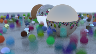
2.6. 整合上述所有内容 下面的代码取自上一本书末尾场景中的漫反射球体示例,并使其在图像渲染过程中移动。每个球体从时间$t=0$时的中心$C$移动到时间$t=1$时的$C+(0,r/2,0)$:
1
2
3
4
5
6
7
8
9
10
11
12
13
14
15
16
17
18
19
20
21
22
23
24
25
26
27
28
29
30
31
32
33
34
35
36
37
38
39
40
41
42
int main () hittable_list world; auto ground_material = make_shared <lambertian>(color (0.5 , 0.5 , 0.5 )); world.add (make_shared <sphere>(point3 (0 ,-1000 ,0 ), 1000 , ground_material)); for (int a = -11 ; a < 11 ; a++) { for (int b = -11 ; b < 11 ; b++) { auto choose_mat = random_double (); point3 center (a + 0.9 *random_double(), 0.2 , b + 0.9 *random_double()) ; if ((center - point3 (4 , 0.2 , 0 )).length () > 0.9 ) { shared_ptr<material> sphere_material; if (choose_mat < 0.8 ) { auto albedo = color::random () * color::random (); sphere_material = make_shared <lambertian>(albedo); auto center2 = center + vec3 (0 , random_double (0 ,.5 ), 0 ); world.add (make_shared <sphere>(center, center2, 0.2 ,sphere_material)); } else if (choose_mat < 0.95 ) { ... } ... camera cam; cam.aspect_ratio = 16.0 / 9.0 ; cam.image_width = 400 ; cam.samples_per_pixel = 100 ; cam.max_depth = 50 ; cam.vfov = 20 ; cam.lookfrom = point3 (13 ,2 ,3 ); cam.lookat = point3 (0 ,0 ,0 ); cam.vup = vec3 (0 ,1 ,0 ); cam.defocus_angle = 0.6 ; cam.focus_dist = 10.0 ; cam.render (world); }
渲染结果如下:
3. 层次包围盒(BVH) 这部分是我们正在开发的光线追踪渲染器中迄今为止最困难和最复杂的部分。我把它放在这一章中,这样代码就可以运行得更快。在这里要稍微重构一下hittable,当我添加矩形和立方体时,我们就不用再重新重构它们了。
光线与物体的交点是光线追踪渲染器的主要时间瓶颈,运行时间与物体数量呈线性关系。但这是对同一场景的重复搜索,因此我们应该能够按照二分搜索的精神使其成为对数搜索。因为我们将数百万到数十亿条光线发送到同一场景,所以我们可以对场景中的物体进行排序,然后每个光线交点都可以进行次线性搜索。两种最常见的排序方法是 1) 划分子空间,2) 划分子物体。后者通常更容易编写代码,并且对于大多数模型来说运行速度同样快。
3.1. 关键思想 为一组基本图元创建包围体积的关键思想是找到一个完全包围所有对象的体积。例如,假设您计算了一个包含10 个对象的球体。任何未击中包围盒的射线肯定会错过里面的所有十个对象。如果射线击中包围盒,那么它可能会击中十个对象中的一个。因此,边界代码始终采用以下形式:
1
2
3
4
if (ray hits bounding object) return whether ray hits bounded objects else return false
请注意,我们将使用这些包围体积组织场景中的对象,将其划分到为子组内。我们不会划分屏幕或场景空间。我们希望任何给定的对象都只位于一个包围盒中,尽管包围盒可能会重叠。
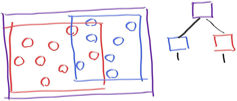
3.2. 层次包围盒 为了使事物次线性化,我们需要创建包围盒。例如,如果我们将一组对象分为两组,红色和蓝色,并使用矩形包围盒,我们将得到:
请注意,蓝色和红色的包围盒包含在紫色包围盒中,但它们可能会重叠,而且它们没有排序——它们只是被包含在里面。因此,右侧显示的树没有左子节点和右子节点排序的概念。它们只是包含关系。代码如下:
1
2
3
4
5
6
if (hits purple) hit0 = hits blue enclosed objects hit1 = hits red enclosed objects if (hit0 or hit1) return true and info of closer hit return false
3.3. 轴对齐包围盒(AABB) 为了使这一切发挥作用,我们需要一种方法来做出好的划分,而不是糟糕的划分,以及一种方法来计算射线与包围盒的相交。射线-包围盒的相交过程需要快速,包围盒需要非常紧凑。在实践中,对于大多数模型,AABB比其他的选择(例如上面提到的球形包围盒)效果更好,但如果您遇到其他类型的包围盒模型,这种设计选择始终是需要牢记的。
从现在开始,我们将轴对齐的长方体(实际上,如果我们要精确地称呼它们,就应该这样称呼)称为AABB。(在代码中,您还会遇到“边界框”的命名缩写“bbox”。)任何您想用来将射线与AABB相交的方法都可以。我们需要知道的只是我们是否击中了它。我们不需要击中点或法线或任何显示对象所需的东西。
大多数人使用“平板”方法。这是基于这样的观察:$n$维AABB只是$n$个正交对齐轴区间的交点,通常称为“平板”。回想一下,区间只是两个端点内的点,例如,范围$3≤x≤5$,或者更简洁地说是$[3,5]$。在 2D 中,AABB(矩形)由两个间隔的重叠定义:
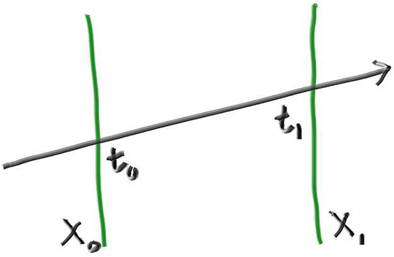
要确定射线是否击中一个区间,我们首先需要确定射线是否击中边界。例如,在一维中,射线与两个平面相交将产生射线参数$t_0$和$t_1$。(如果射线平行于平面,则它与任何平面的交点都将无法确定。)
我们如何找到射线和平面之间的交点?回想一下,射线只是由一个函数定义的,该函数给定一个参数$t$,并返回一个位置$P(t)$:
将这个等式应用到x,y,z三个分量上。例如$x(t)=Q_x+td_x$。当射线与平面$x=x_0$相交时,存在参数$t$满足下面的方程:
因此交点的$t$为
对于$x_1$,可以获得相似的结论:
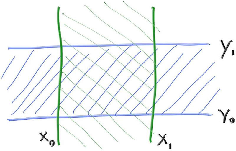
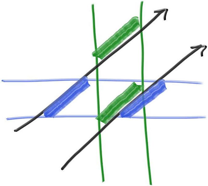
将一维数学转化为二维或三维命中的关键结论是:如果射线与构成包围盒相交,则射线的所有构成包围盒的平面相交$t$值区间将重叠。例如,在二维中,只有当射线与AABB相交时,才会发生绿色和蓝色重叠:
在此图中,上方的射线间隔不重叠,因此我们知道射线没有击中绿色和蓝色平面所包围的2D AABB。下方的射线间隔确实重叠,因此我们知道下方的射线确实击中了AABB。
3.4. 射线与AABB相交 以下伪代码确定”平板”中的$t$区间是否重叠:
1
2
3
interval_x ← compute_intersection_x (ray, x0, x1) interval_y ← compute_intersection_y (ray, y0, y1) return overlaps (interval_x, interval_y)
这非常简单,而且3D版本可以很容易基于上面的内容扩展,这就是人们喜欢平面相交法的原因:
1
2
3
4
interval_x ← compute_intersection_x (ray, x0, x1) interval_y ← compute_intersection_y (ray, y0, y1) interval_z ← compute_intersection_z (ray, z0, z1) return overlaps (interval_x, interval_y, interval_z)
有一些注意事项使得它看起来并不那么漂亮。再次考虑$t_0$和$t_1$的一维方程:
第一,假设射线指向着$x$轴负方向。区间$(t_{x_0}, t_{x_1})$可能会翻转,例如$(7,3)$。第二,分子$d_x$可能为0,这会产生一个无穷大的数。并且,当射线的起点在边界上时,我们会计算出$NaN$,因为分子分母都为0了。此外,IEEE 标准定义的浮点数,可能会有$\pm 0$的情况。
对于$d_x=0$来说,好消息是$t_{x_0}$ 和$t_{x_1}$ 将相等:如果$x_0$和$x_1$之间不相等,则均为$+\infin$或$-\infin$。因此,使用$min$和$max$应该可以得到正确的答案:
还剩下一个麻烦是如果$d_x= 0$和这两种情况同时发生:$x_0-Q_x=0$或$x_1-Q_x=0$,将会得到$NaN$的结果。在这种情况下,我们可以将其解释为命中或未命中,我们稍后会重新讨论这一点。
现在,让我们来看overlaps的伪代码。我们可以假设区间不是反转的,并且我们希望区间重叠时返回true。boolean Overlaps()函数计算$t_{interval\space1}$和$t_{interval\space 2}$的重叠区间$t$,并判断该区间是否为空。
1
2
3
4
bool overlaps (t_interval1, t_interval2) t_min ← max (t_interval1. min, t_interval2. min) t_max ← min (t_interval1. max, t_interval2. max) return t_min < t_max
如果上面的过程有$NaN$的情况,比较结果将返回false,因此我们需要给我们的包围盒添加一个微小的padding。(我们最好这样做,因为在光线追踪渲染器中说明情况都可能出现)
为了实现这一点,我们首先添加一个新的区间函数expand,它按给定的值扩充区间:
1
2
3
4
5
6
7
8
9
10
11
12
13
14
15
16
class interval { public : ... double clamp (double x) const if (x < min) return min; if (x > max) return max; return x; } interval expand (double delta) const { auto padding = delta/2 ; return interval (min - padding, max + padding); } static const interval empty, universe; };
现在我们已经拥有实现AABB类所需的一切。
1 2 3 4 5 6 7 8 9 10 11 12 13 14 15 16 17 18 19 20 21 22 23 24 25 26 27 28 29 30 31 32 33 34 35 36 37 38 39 40 41 42 43 44 45 46 47 48 49 50 51 52 53 54 #ifndef AABB_H #define AABB_H class aabb { public : interval x, y, z; aabb () {} aabb (const interval& x, const interval& y, const interval& z) : x (x), y (y), z (z) {} aabb (const point3& a, const point3& b) { x = (a[0 ] <= b[0 ]) ? interval (a[0 ], b[0 ]) : interval (b[0 ], a[0 ]); y = (a[1 ] <= b[1 ]) ? interval (a[1 ], b[1 ]) : interval (b[1 ], a[1 ]); z = (a[2 ] <= b[2 ]) ? interval (a[2 ], b[2 ]) : interval (b[2 ], a[2 ]); } const interval& axis_interval (int n) const if (n == 1 ) return y; if (n == 2 ) return z; return x; } bool hit (const ray& r, interval ray_t ) const const point3& ray_orig = r.origin (); const vec3& ray_dir = r.direction (); for (int axis = 0 ; axis < 3 ; axis++) { const interval& ax = axis_interval (axis); const double adinv = 1.0 / ray_dir[axis]; auto t0 = (ax.min - ray_orig[axis]) * adinv; auto t1 = (ax.max - ray_orig[axis]) * adinv; if (t0 < t1) { if (t0 > ray_t .min) ray_t .min = t0; if (t1 < ray_t .max) ray_t .max = t1; } else { if (t1 > ray_t .min) ray_t .min = t1; if (t0 < ray_t .max) ray_t .max = t0; } if (ray_t .max <= ray_t .min) return false ; } return true ; } }; #endif
3.5. 在Hittables中构造AABB 我们现在需要添加一个函数来计算所有Hittables对象的包围盒。然后,我们将在所有图元上创建一个包围盒的层次结构(BVH),并且各个图元(如球体)将位于叶子节点上。
回想一下,默认情况下,没有参数构造的interval的值将为空。由于AABB对象的三个实例都有一个interval,因此默认情况下每个实例都将为空,因此AABB对象默认情况下将为空。因此,某些对象可能具有空的包围盒。例如,一个没有子节点的hittable_list对象。令人高兴的是,我们设计interval类时考虑了这些,数学上一切都说得通。
最后,回想一下,某些对象可能是运动的。此类对象应返回其在整个运动范围内(从$time=0$到$time=1$)的包围盒。
1 2 3 4 5 6 7 8 9 #include "aabb.h" class material ;... class hittable { public : virtual ~hittable () = default ; virtual bool hit (const ray& r, interval ray_t , hit_record& rec) const 0 ; virtual aabb bounding_box () const 0 ; }
对于静止的球体,bounding_box的功能很简单:
1
2
3
4
5
6
7
8
9
10
11
12
13
14
15
16
17
18
class sphere : public hittable { public : sphere (const point3& static_center, double radius, shared_ptr<material> mat) : center (static_center, vec3 (0 ,0 ,0 )), radius (std::fmax (0 ,radius)), mat (mat) { auto rvec = vec3 (radius, radius, radius); bbox = aabb (static_center - rvec, static_center + rvec); } ... aabb bounding_box () const override { return bbox; } private : ray center; double radius; shared_ptr<material> mat; aabb bbox; ... };
对于移动的球体,我们需要其整个运动范围的包围盒。为此,我们可以取$time=0$的包围盒和$time=1$的包围盒,并计算这包围这两个包围盒的包围盒。
1
2
3
4
5
6
7
8
9
10
11
12
13
14
class sphere : public hittable { public : ... sphere (const point3& center1, const point3& center2, double radius, shared_ptr<material> mat) : center (center1, center2 - center1), radius (std::fmax (0 ,radius)), mat (mat) { auto rvec = vec3 (radius, radius, radius); aabb box1 (center.at(0 ) - rvec, center.at(0 ) + rvec) ; aabb box2 (center.at(1 ) - rvec, center.at(1 ) + rvec) ; bbox = aabb (box1, box2); } ... };
现在我们需要一个新的AABB构造函数,它将两个AABB作为输入。首先,我们将添加新的interval构造函数来执行此操作:
1
2
3
4
5
6
7
8
9
10
11
12
13
class interval { public : double min, max; interval () : min (+infinity), max (-infinity) {} interval (double _min, double _max) : min (_min), max (_max) {} interval (const interval& a, const interval& b) { min = a.min <= b.min ? a.min : b.min; max = a.max >= b.max ? a.max : b.max; } double size () const ...
现在我们可以使用它来从两个输入的AABB构造一个AABB包围盒。
1
2
3
4
5
6
7
8
9
10
11
12
13
class aabb { public : ... aabb (const point3& a, const point3& b) { ... } aabb (const aabb& box0, const aabb& box1) { x = interval (box0. x, box1. x); y = interval (box0. y, box1. y); z = interval (box0. z, box1. z); } ... };
3.6. 创建物体列表的包围盒 现在我们将更新hittable_list对象,计算其子对象的包围盒。我们将在每添加一个新子对象时逐步更新包围盒。
1 2 3 4 5 6 7 8 9 10 11 12 13 14 15 16 17 18 19 #include "aabb.h" #include "hittable.h" #include <vector> class hittable_list : public hittable { public : std::vector<shared_ptr<hittable>> objects; ... void add (shared_ptr<hittable> object) objects.push_back (object); bbox = aabb (bbox, object->bounding_box ()); } bool hit (const ray& r, interval ray_t , hit_record& rec) const override ... } aabb bounding_box () const override { return bbox; } private : aabb bbox; };
3.7. BVH的节点类 BVH也将是一个Hittable对象——就像Hittable_list一样。它实际上是一个容器,但它可以响应查询:一束光线是否击中了它。目前存在一个问题,就是我们是否需要两个类,一个用于树,一个用于树中的节点。或者说,我们是否仅仅需要一个类,并且根只是我们指向的一个节点。命中函数非常简单:判断节点的包围盒与射线是否相交,如果是,则递归地判断子节点是否与射线相交。
我热衷于第二种方法,下面是代码实现:
1 2 3 4 5 6 7 8 9 10 11 12 13 14 15 16 17 18 19 20 21 22 23 24 25 26 27 28 29 30 31 32 33 34 35 36 37 38 39 #ifndef BVH_H #define BVH_H #include "aabb.h" #include "hittable.h" #include "hittable_list.h" class bvh_node : public hittable { public : bvh_node (hittable_list list) : bvh_node (list.objects, 0 , list.objects.size ()) { } bvh_node (std::vector<shared_ptr<hittable>>& objects, size_t start, size_t end) { } bool hit (const ray& r, interval ray_t , hit_record& rec) const override if (!bbox.hit (r, ray_t )) return false ; bool hit_left = left->hit (r, ray_t , rec); bool hit_right = right->hit (r, interval (ray_t .min, hit_left ? rec.t : ray_t .max), rec); return hit_left || hit_right; } aabb bounding_box () const override { return bbox; } private : shared_ptr<hittable> left; shared_ptr<hittable> right; aabb bbox; }; #endif
3.8. 划分BVH包围体积 任何加速结构(包括 BVH)最复杂的部分是构建它。我们在构造函数中执行此操作。BVH 的一个很酷的地方是,只要bvh_node中的对象列表被分成两个子列表,命中函数就会起作用。如果划分做得好,效果会最好,这样两个子节点的包围盒就会比其父节点的包围盒小,但这是为了速度而不是为了正确性。我将选择折衷方案,并在每个节点沿一个轴分割对象列表。我会选择简单的方案:
随机选择划分轴
对图元进行排序(使用std::sort)
对半分开,分别放入左右子树
当传入的列表只有两个元素时,我会在每个子树中各放入一个元素并结束递归。遍历算法应该是丝滑的,并且不必检查空指针,因此,若我只有一个元素,我会在每个子树中复制它。明确检查三个元素并只进行一次递归可能会比较好,但我认为整个方法稍后会得到优化。以下代码使用了我们尚未定义的三个方法box_x_compare、box_y_compare和box_z_compare。
1 2 3 4 5 6 7 8 9 10 11 12 13 14 15 16 17 18 19 20 21 22 23 24 25 26 27 28 29 30 31 32 33 34 35 36 37 #include "aabb.h" #include "hittable.h" #include "hittable_list.h" #include <algorithm> class bvh_node : public hittable { public : ... bvh_node (std::vector<shared_ptr<hittable>>& objects, size_t start, size_t end) { int axis = random_int (0 ,2 ); auto comparator = (axis == 0 ) ? box_x_compare : (axis == 1 ) ? box_y_compare : box_z_compare; size_t object_span = end - start; if (object_span == 1 ) { left = right = objects[start]; } else if (object_span == 2 ) { left = objects[start]; right = objects[start+1 ]; } else { std::sort (std::begin (objects) + start, std::begin (objects) + end,comparator); auto mid = start + object_span/2 ; left = make_shared <bvh_node>(objects, start, mid); right = make_shared <bvh_node>(objects, mid, end); } bbox = aabb (left->bounding_box (), right->bounding_box ()); } ... };
这是新函数的定义:random_int():
1
2
3
4
5
6
7
8
9
10
11
12
13
... inline double random_double (double min, double max) return min + (max-min)*random_double (); } inline int random_int (int min, int max) return int (random_double (min, max+1 )); } ...
检查是否存在包围盒是为了防止你实现了没有包围盒的,类似无限平面的几何图元。我们没有实现这种图元,所以除非你自己添加这样的东西,否则这种情况不会发生。
3.9. 比较函数: 现在我们需要实现std::sort()使用的比较函数。为此,创建一个通用的比较器,如果第一个参数小于第二个参数,则返回 true,并指定参数表示轴。然后定义各个轴特定的比较函数。
1
2
3
4
5
6
7
8
9
10
11
12
13
14
15
16
17
18
19
20
21
22
23
24
25
26
27
28
29
class bvh_node : public hittable { ... private : shared_ptr<hittable> left; shared_ptr<hittable> right; aabb bbox; static bool box_compare ( const shared_ptr<hittable> a, const shared_ptr<hittable> b, int axis_index ) auto a_axis_interval = a->bounding_box ().axis_interval (axis_index); auto b_axis_interval = b->bounding_box ().axis_interval (axis_index); return a_axis_interval.min < b_axis_interval.min; } static bool box_x_compare (const shared_ptr<hittable> a, const shared_ptr<hittable> b) return box_compare (a, b, 0 ); } static bool box_y_compare (const shared_ptr<hittable> a, const shared_ptr<hittable> b) return box_compare (a, b, 1 ); } static bool box_z_compare (const shared_ptr<hittable> a, const shared_ptr<hittable> b) return box_compare (a, b, 2 ); } };
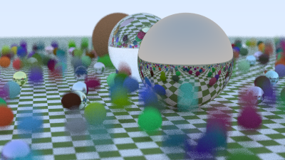
此时,我们已准备好使用新的 BVH 代码。让我们在随机球体场景中使用它。
1 2 3 4 5 6 7 8 9 10 11 12 13 14 15 16 17 18 19 20 21 22 23 24 #include "rtweekend.h" #include "bvh.h" #include "camera.h" #include "hittable.h" #include "hittable_list.h" #include "material.h" #include "sphere.h" int main () ... auto material2 = make_shared <lambertian>(color (0.4 , 0.2 , 0.1 )); world.add (make_shared <sphere>(point3 (-4 , 1 , 0 ), 1.0 , material2)); auto material3 = make_shared <metal>(color (0.7 , 0.6 , 0.5 ), 0.0 ); world.add (make_shared <sphere>(point3 (4 , 1 , 0 ), 1.0 , material3)); world = hittable_list (make_shared <bvh_node>(world)); camera cam; ... }
渲染后的图像应与图 1 中所示的非BVH版本相同。但是,如果对两个版本进行计时,BVH版本应该更快。我发现速度几乎是之前版本的六倍半。
3.10. BVH的其他优化 我们可以稍微加快BVH优化的速度。我们不要选择随机分割轴,而是分割包围盒的最长轴以获得最大的划分。这个改变很简单,但我们会在此过程中向aabb类添加一些内容。
第一个是在BVH构造函数中构造一个包含所有划分对象的AABB。方法是将AABB初始化为空(我们将很快定义aabb::empty),然后用对象列表中的每个AABB对其进行扩充。
一旦我们有了AABB,就将分割轴设置为边最长的轴。我们设想一个函数来为我们做这件事:aabb::longest_axis()。最后,由于我们预先计算了包含所有对象的AABB,我们可以删除原来合并左右两个子包围盒为一个包围盒的代码。
1
2
3
4
5
6
7
8
9
10
11
12
13
14
15
16
17
18
19
20
21
class bvh_node : public hittable { public : ... bvh_node (std::vector<shared_ptr<hittable>>& objects, size_t start, size_t end) { bbox = aabb::empty; for (size_t object_index=start; object_index < end; object_index++) bbox = aabb (bbox, objects[object_index]->bounding_box ()); int axis = bbox.longest_axis (); auto comparator = (axis == 0 ) ? box_x_compare : (axis == 1 ) ? box_y_compare : box_z_compare; ... } ...
现在实现空的aabb代码和新的aabb::longest_axis()函数:
1
2
3
4
5
6
7
8
9
10
11
12
13
14
15
16
17
18
19
20
21
22
class aabb { public : ... bool hit (const ray& r, interval ray_t ) const ... } int longest_axis () const if (x.size () > y.size ()) return x.size () > z.size () ? 0 : 2 ; else return y.size () > z.size () ? 1 : 2 ; } static const aabb empty, universe; }; const aabb aabb::empty = aabb (interval::empty, interval::empty, interval::empty);const aabb aabb::universe = aabb (interval::universe, interval::universe, interval::universe);
与之前一样,您应该看到与图 1相同的结果,但渲染速度稍快一些。在我的系统上,这会产生大约18%的额外渲染速度。对于一点额外的工作来说,这还不错。
4. 纹理映射 计算机图形学中的纹理映射(Texture Mapping)是将材质效果应用于场景中的对象的过程。“纹理”部分是效果,“映射”部分在数学上是将一个空间映射到另一个空间。这种效果可以是任何材质属性:颜色、光泽度、凹凸几何形状(称为“凹凸映射”),甚至是材质的显隐(用于创建表面的剪切区域)。
最常见的纹理映射类型是将图像映射到物体表面上,定义物体表面上每个点的颜色。实际上,我们以相反的方式实现该过程:给定物体上的某个点,我们将查找纹理映射定义的颜色。
首先,我们将使纹理颜色程序化,并创建一个以常量颜色构成的纹理图。大多数程序将恒定的RGB颜色和纹理保留在不同的类中,因此你可以随意做些不同的事情,而我也非常喜欢这种架构,因为能够将任何颜色变成纹理真是太棒了。
为了执行纹理查找,我们需要一个纹理坐标 。这个坐标可以用多种方式定义,我们将在开发过程中逐步讨论它的实现方式。现在,我们将传入二维纹理坐标。按照惯例,纹理坐标命名为$u$和$v$。对于恒定纹理,每个$(u,v)$对都会产生恒定颜色,因此我们实际上可以完全忽略坐标。但是,其他纹理类型将需要这些坐标,因此我们将它们保存在方法接口中。
我们的纹理类的主要方法是color value(...)方法,该方法根据输入坐标返回纹理颜色。除了获取点的纹理坐标$u$和$v$ 之外,我们还提供相关点的位置,原因稍后会说明。
4.1. 常数颜色纹理 1 2 3 4 5 6 7 8 9 10 11 12 13 14 15 16 17 18 19 20 21 22 23 24 25 #ifndef TEXTURE_H #define TEXTURE_H class texture { public : virtual ~texture () = default ; virtual color value (double u, double v, const point3& p) const 0 ; }; class solid_color : public texture { public : solid_color (const color& albedo) : albedo (albedo) {} solid_color (double red, double green, double blue) : solid_color (color (red,green,blue)) {} color value (double u, double v, const point3& p) const override { return albedo; } private : color albedo; }; #endif
我们需要更新hit_record结构来存储命中点的$u,v$表面坐标。
1 2 3 4 5 6 7 8 9 10 11 class hit_record { public : vec3 p; vec3 normal; shared_ptr<material> mat; double t; double u; double v; bool front_face; ...
将来,我们需要计算每种hittable类型上给定点的$(u,v)$纹理坐标。稍后会详细介绍。
4.2. 实体纹理:棋盘格纹理 实体(或空间)纹理仅取决于3D空间中每个点的位置。你可以将实体纹理想象为给空间本身中的所有点着色,而不是给该空间中的特定对象着色。因此,对象可以在改变位置时改变纹理映射的结果,尽管你通常会将对象和实体纹理进行绑定。
为了探讨空间纹理,我们将实现一个空间checker_texture类,该类实现三维棋盘格图案。由于空间纹理函数由空间中的给定位置驱动,因此纹理“value()”函数会忽略u和v参数,而仅使用参数p。
为了实现方格图案,我们首先要计算输入点每个分量的底数。我们可以截断坐标,但这会将值拉向零,从而导致零的两边颜色相同。底数函数始终将值移到左侧的整数值(向负无穷大方向)。给定这三个整数结果$(\lfloor x \rfloor,\lfloor y\rfloor,\lfloor z\rfloor)$,我们取它们的和并计算结果模2,结果为0或1。0映射到偶数颜色,1映射到奇数颜色。
最后,我们给纹理添加一个缩放因子,以便我们控制场景中棋盘图案的大小。
1 2 3 4 5 6 7 8 9 10 11 12 13 14 15 16 17 18 19 20 21 22 23 class checker_texture : public texture { public : checker_texture (double scale, shared_ptr<texture> even, shared_ptr<texture> odd) : inv_scale (1.0 / scale), even (even), odd (odd) {} checker_texture (double scale, const color& c1, const color& c2) : checker_texture (scale, make_shared <solid_color>(c1), make_shared <solid_color>(c2)) {} color value (double u, double v, const point3& p) const override { auto xInteger = int (std::floor (inv_scale * p.x ())); auto yInteger = int (std::floor (inv_scale * p.y ())); auto zInteger = int (std::floor (inv_scale * p.z ())); bool isEven = (xInteger + yInteger + zInteger) % 2 == 0 ; return isEven ? even->value (u, v, p) : odd->value (u, v, p); } private : double inv_scale; shared_ptr<texture> even; shared_ptr<texture> odd; };
这些棋盘奇偶参数可以指向一个常量纹理或其他程序纹理。这体现了Pat Hanrahan在 20 世纪 80 年代引入的着色器网络的精神。
为了支持程序纹理,我们将扩展lambertian类以使用纹理而不是颜色:
1 2 3 4 5 6 7 8 9 10 11 12 13 14 15 16 17 18 19 20 21 22 23 24 25 26 #include "hittable.h" #include "texture.h" ... class lambertian : public material { public : lambertian (const color& albedo) : tex (make_shared <solid_color>(albedo)) {} lambertian (shared_ptr<texture> tex) : tex (tex) {} bool scatter (const ray& r_in, const hit_record& rec, color& attenuation, ray& scattered) const override { auto scatter_direction = rec.normal + random_unit_vector (); if (scatter_direction.near_zero ()) scatter_direction = rec.normal; scattered = ray (rec.p, scatter_direction, r_in.time ()); attenuation = tex->value (rec.u, rec.v, rec.p); return true ; } private : shared_ptr<texture> tex; };
如果我们将其添加到我们的主要场景:
1 2 3 4 5 6 7 8 9 10 11 12 13 14 15 16 17 18 19 20 #include "rtweekend.h" #include "bvh.h" #include "camera.h" #include "hittable.h" #include "hittable_list.h" #include "material.h" #include "sphere.h" #include "texture.h" int main () hittable_list world; auto checker = make_shared <checker_texture>(0.32 , color (.2 , .3 , .1 ), color (.9 , .9 , .9 )); world.add (make_shared <sphere>(point3 (0 ,-1000 ,0 ), 1000 , make_shared <lambertian>(checker))); for (int a = -11 ; a < 11 ; a++) { ... }
渲染结果如下:
4.3. 渲染实体棋盘格纹理 我们将在程序中添加第二个场景,之后随着本书的进展,我们将添加更多场景。为了便于实现这一点,我们将设置一个switch语句来为单词运行选择所需的场景。这是一种粗糙的实现方法,但我们试图让事情变得非常简单,并专注于光线追踪算法本身。您可能希望在自己的光线追踪器中使用不同的方法来实现这一点,例如使用命令行参数。
以下是针对单个随机球体场景重构后的main.cc。将main()重命名为bouncing_spheres(),并添加一个新的 main() 函数来调用它
1 2 3 4 5 6 7 8 9 10 11 12 13 14 15 16 17 18 19 20 21 22 23 24 25 #include "rtweekend.h" #include "bvh.h" #include "camera.h" #include "hittable.h" #include "hittable_list.h" #include "material.h" #include "sphere.h" #include "texture.h" void bouncing_spheres () hittable_list world; auto ground_material = make_shared <lambertian>(color (0.5 , 0.5 , 0.5 )); world.add (make_shared <sphere>(point3 (0 ,-1000 ,0 ), 1000 , ground_material)); ... cam.render (world); } int main () bouncing_spheres (); }
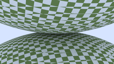
现在,增加要给有两个棋盘格球体的场景,一个在顶部,另一个在底部。
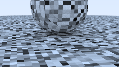
1 2 3 4 5 6 7 8 9 10 11 12 13 14 15 16 17 18 19 20 21 22 23 24 25 26 27 28 29 30 31 32 33 34 35 36 37 38 39 40 41 42 43 44 45 46 #include "rtweekend.h" #include "bvh.h" #include "camera.h" #include "hittable.h" #include "hittable_list.h" #include "material.h" #include "sphere.h" #include "texture.h" void bouncing_spheres () ... } void checkered_spheres () hittable_list world; auto checker = make_shared <checker_texture>(0.32 , color (.2 , .3 , .1 ), color (.9 , .9 , .9 )); world.add (make_shared <sphere>(point3 (0 ,-10 , 0 ), 10 , make_shared <lambertian>(checker))); world.add (make_shared <sphere>(point3 (0 , 10 , 0 ), 10 , make_shared <lambertian>(checker))); camera cam; cam.aspect_ratio = 16.0 / 9.0 ; cam.image_width = 400 ; cam.samples_per_pixel = 100 ; cam.max_depth = 50 ; cam.vfov = 20 ; cam.lookfrom = point3 (13 ,2 ,3 ); cam.lookat = point3 (0 ,0 ,0 ); cam.vup = vec3 (0 ,1 ,0 ); cam.defocus_angle = 0 ; cam.render (world); } int main () switch (2 ) { case 1 : bouncing_spheres (); break ; case 2 : checkered_spheres (); break ; } }
渲染结果如下:
您可能认为结果看起来有点奇怪。由于checker_texture是空间纹理,我们实际上看到的是球体表面穿过三维棋盘空间。在很多情况下,这是完美的,或者至少是足够的。在许多其他情况下,我们确实希望在物体表面上获得一致的效果。接下来将介绍这种方法。
4.4. 球体纹理坐标 恒定颜色纹理不使用坐标。实体(或空间)纹理使用空间中某个点的坐标。现在是时候使用$u,v$纹理坐标了。这些坐标指定2D源图像(或某个2D参数化空间)上的位置。为此,我们需要一种方法来计算3D物体表面上任何点的$u,v$坐标。这种映射完全是任意的,但通常您希望覆盖整个表面,并能够以某种合理的方式缩放、定位和拉伸2D图像。我们将从一个简单的方案开始,逐步介绍如何获取球体的$u,v$坐标。
对于球体,纹理坐标通常基于某种形式的经度和纬度,即球面坐标。因此,我们在球面坐标中计算$(\theta,\phi)$,其中$\theta$是从底极向上的角度(即从$-Y$向上),$\phi$是围绕$Y$轴的角度(从$-X$到$+Z$再到$+X$再到$-Z$回到$-X$)。
我们想要把$\theta$和$\phi$映射到纹理坐标$u$和$v$上,$u,v$的取值范围是$[0,1]$。当$(u=0,v=0)$时,映射到纹理的左下角。这样一来,映射公式就可以被定义如下:
为了计算以原点为中心的单位球面上给定点的$\theta$和$\phi$,我们从相应的笛卡尔坐标方程开始:
为了求解$\theta$和$\phi$,需要将上面的等式变形。得益于<cmath>中定义的std::atan2()函数,我们可以把$x$和$z$传进去来求解$\phi$,该函数接受成任意一对正弦和余弦的值并返回对应的弧度(方位角)。
std::atan2()的返回值的范围是$[-\pi,\pi]$,但是在$\pi$和$-\pi$的取值是突变的。虽然这在数学上是正确的,但是我们希望$u$的取值范围是0到1,而不是0到0.5,然后从-0.5到0。幸运的是:
第二个方程输出的值是连续地从0到$2\pi$。这样,我们可以基于下面地公式计算出$\phi$:
对于$(u,v)$坐标,可以通过通用函数来计算,传入以原点为圆心的单位球表面的点,输出$(u,v)$坐标。
1 2 3 4 5 6 7 8 9 10 11 12 13 14 15 16 17 18 19 20 class sphere : public hittable { ... private : ... static void get_sphere_uv (const point3& p, double & u, double & v) auto theta = std::acos (-p.y ()); auto phi = std::atan2 (-p.z (), p.x ()) + pi; u = phi / (2 *pi); v = theta / pi; } };
更新sphere::hit()函数,并引用上面的函数来计算UV坐标:
1 2 3 4 5 6 7 8 9 10 11 12 13 14 15 16 17 class sphere : public hittable { public : ... bool hit (const ray& r, interval ray_t , hit_record& rec) const override ... rec.t = root; rec.p = r.at (rec.t); vec3 outward_normal = (rec.p - current_center) / radius; rec.set_face_normal (r, outward_normal); get_sphere_uv (outward_normal, rec.u, rec.v); rec.mat = mat; return true ; } ... };
基于碰撞点$P$,我们计算了表面的UV坐标。后续将使用该坐标去索引我们程序生成的实体纹理(如大理石)。我们还可以读取一张图片,并使用2D$(u,v)$去采样这张图片。
在图像中使用缩放的$(u,v)$的直接方法是将$u$和$v$四舍五入为整数,并将其用作$(i,j)$像素。这很尴尬,因为我们不想在更改图像分辨率时更改代码。因此,图形中最通用的非官方标准之一是使用纹理坐标而不是图像像素坐标。这些只是图像像素位置的某种表现形式。例如,对于$N_x$X$N_y$的图像中,像素$(i,j)$,图像纹理位置为:
相应地,可以从$(u,v)$计算出$(i,j)$。
4.5. 访问纹理图片数据 现在,是时候创建表示图片纹理的类了。我将会使用我喜欢的图形库:stb_image 。它可以读取图片数据并保存在32位浮点数数组中。这些数据表示RGB的值的每一个分量,且范围是$[0,1]$(由黑到纯白)。此外,图片被加载到线性空间中(gamma=1),能够适配我们前面所作的所有计算。
为了让加载图片更简单,我们提供一个辅助类来管理:rtw_image。它提供了一个辅助函数:pixel_data(int x, int y),通过该函数可以获得指定像素的8-bits RGB值。下面的代码假设你已经把stb_image.h拷贝到一个叫external的文件夹。你可以根据自己的目录结构进行调整。
1 2 3 4 5 6 7 8 9 10 11 12 13 14 15 16 17 18 19 20 21 22 23 24 25 26 27 28 29 30 31 32 33 34 35 36 37 38 39 40 41 42 43 44 45 46 47 48 49 50 51 52 53 54 55 56 57 58 59 60 61 62 63 64 65 66 67 68 69 70 71 72 73 74 75 76 77 78 79 80 81 82 83 84 85 86 87 88 89 90 91 92 93 94 95 96 97 98 99 100 101 102 103 104 105 106 107 108 109 110 111 112 113 114 115 116 117 118 119 120 121 122 123 124 125 126 #ifndef RTW_STB_IMAGE_H #define RTW_STB_IMAGE_H #ifdef _MSC_VER #pragma warning (push, 0) #endif #define STB_IMAGE_IMPLEMENTATION #define STBI_FAILURE_USERMSG #include "external/stb_image.h" #include <cstdlib> #include <iostream> class rtw_image { public : rtw_image () {} rtw_image (const char * image_filename) { auto filename = std::string (image_filename); auto imagedir = getenv ("RTW_IMAGES" ); if (imagedir && load (std::string (imagedir) + "/" + image_filename)) return ; if (load (filename)) return ; if (load ("images/" + filename)) return ; if (load ("./img/images/" + filename)) return ; if (load (".././img/images/" + filename)) return ; if (load ("../.././img/images/" + filename)) return ; if (load ("../../.././img/images/" + filename)) return ; if (load ("../../../.././img/images/" + filename)) return ; if (load ("../../../../.././img/images/" + filename)) return ; std::cerr << "ERROR: Could not load image file '" << image_filename << "'.\n" ; } ~rtw_image () { delete [] bdata; STBI_FREE (fdata); } bool load (const std::string& filename) auto n = bytes_per_pixel; fdata = stbi_loadf (filename.c_str (), &image_width, &image_height, &n, bytes_per_pixel); if (fdata == nullptr ) return false ; bytes_per_scanline = image_width * bytes_per_pixel; convert_to_bytes (); return true ; } int width () const return (fdata == nullptr ) ? 0 : image_width; } int height () const return (fdata == nullptr ) ? 0 : image_height; } const unsigned char * pixel_data (int x, int y) const static unsigned char magenta[] = { 255 , 0 , 255 }; if (bdata == nullptr ) return magenta; x = clamp (x, 0 , image_width); y = clamp (y, 0 , image_height); return bdata + y*bytes_per_scanline + x*bytes_per_pixel; } private : const int bytes_per_pixel = 3 ; float *fdata = nullptr ; unsigned char *bdata = nullptr ; int image_width = 0 ; int image_height = 0 ; int bytes_per_scanline = 0 ; static int clamp (int x, int low, int high) if (x < low) return low; if (x < high) return x; return high - 1 ; } static unsigned char float_to_byte (float value) if (value <= 0.0 ) return 0 ; if (1.0 <= value) return 255 ; return static_cast <unsigned char >(256.0 * value); } void convert_to_bytes () int total_bytes = image_width * image_height * bytes_per_pixel; bdata = new unsigned char [total_bytes]; auto *bptr = bdata; auto *fptr = fdata; for (auto i=0 ; i < total_bytes; i++, fptr++, bptr++) *bptr = float_to_byte (*fptr); } }; #ifdef _MSC_VER #pragma warning (pop) #endif #endif
如果你使用C/C++以外的语言实现,则需要找到(或编写)提供类似功能的图像加载库。
使用rtw_image类实现image_texture:
1 2 3 4 5 6 7 8 9 10 11 12 13 14 15 16 17 18 19 20 21 22 23 24 25 26 27 28 29 30 31 #include "rtw_stb_image.h" ... class checker_texture : public texture { ... }; class image_texture : public texture { public : image_texture (const char * filename) : image (filename) {} color value (double u, double v, const point3& p) const override { if (image.height () <= 0 ) return color (0 ,1 ,1 ); u = interval (0 ,1 ).clamp (u); v = 1.0 - interval (0 ,1 ).clamp (v); auto i = int (u * image.width ()); auto j = int (v * image.height ()); auto pixel = image.pixel_data (i,j); auto color_scale = 1.0 / 255.0 ; return color (color_scale*pixel[0 ], color_scale*pixel[1 ], color_scale*pixel[2 ]); } private : rtw_image image; };
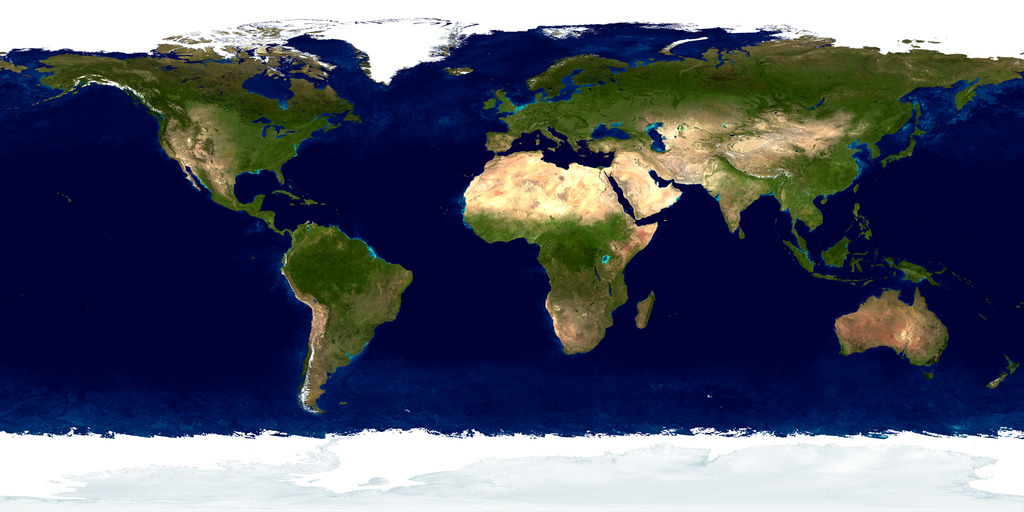
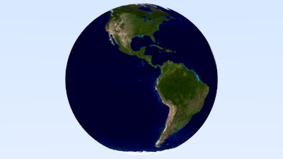
4.6. 渲染图像纹理 我随意从网上找了一张世界地图——任何标准投影都可以满足我们的目的。
下面的代码从文件中读取图片,并将它赋值给材质:
1 2 3 4 5 6 7 8 9 10 11 12 13 14 15 16 17 18 19 20 21 22 23 24 25 26 27 28 29 void earth () auto earth_texture = make_shared <image_texture>("earthmap.jpg" ); auto earth_surface = make_shared <lambertian>(earth_texture); auto globe = make_shared <sphere>(point3 (0 ,0 ,0 ), 2 , earth_surface); camera cam; cam.aspect_ratio = 16.0 / 9.0 ; cam.image_width = 400 ; cam.samples_per_pixel = 100 ; cam.max_depth = 50 ; cam.vfov = 20 ; cam.lookfrom = point3 (0 ,0 ,12 ); cam.lookat = point3 (0 ,0 ,0 ); cam.vup = vec3 (0 ,1 ,0 ); cam.defocus_angle = 0 ; cam.render (hittable_list (globe)); } int main () switch (3 ) { case 1 : bouncing_spheres (); break ; case 2 : checkered_spheres (); break ; case 3 : earth (); break ; } }
我们开始看到把所有颜色都描述为纹理的威力——我们可以为Lambertian材质分配任何类型的纹理,而Lambertian材质只需要从纹理中获取颜色。
如果照片中间有一个大的青色球体,则说明stb_image无法找到你提供的图片路径。程序将在与可执行文件相同的目录中查找该文件。确保将图片复制到您的构建目录中,或重写earth()以指向其他路径。
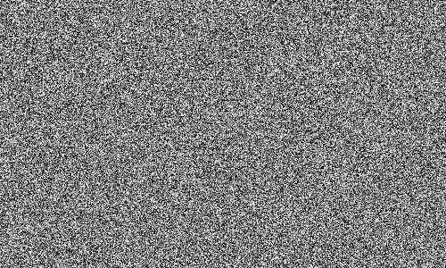
5. 柏林噪声 为了获得看起来很酷的实体纹理,大多数人会使用某种形式的Perlin噪声。这些噪声以其发明者Ken Perlin的名字命名。Perlin纹理不会返回如下白噪声:
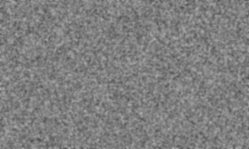
相反,它返回类似于模糊白噪声的东西:
Perlin噪声的一个关键部分是它是可重复的:它以3D顶点作为输入,并始终返回相同的随机数。邻近的点返回类似的数字。Perlin噪声的另一个重要部分是它简单而快速,因此它通常作为一种hack来实现。我将根据Andrew Kensler的描述逐步构建该hack。
5.1. 使用随机数块 我们可以用一个随机数的 3D 数组平铺整个空间,并以块的形式使用它们。你会得到一些块状的东西,其中重复的块是显而易见的:
让我们使用某种哈希来打乱它,而不是平铺。这有一些支持代码来实现这一切:
1 2 3 4 5 6 7 8 9 10 11 12 13 14 15 16 17 18 19 20 21 22 23 24 25 26 27 28 29 30 31 32 33 34 35 36 37 38 39 40 41 42 43 44 45 46 47 48 #ifndef PERLIN_H #define PERLIN_H class perlin { public : perlin () { for (int i = 0 ; i < point_count; i++) { randfloat[i] = random_double (); } perlin_generate_perm (perm_x); perlin_generate_perm (perm_y); perlin_generate_perm (perm_z); } double noise (const point3& p) const auto i = int (4 *p.x ()) & 255 ; auto j = int (4 *p.y ()) & 255 ; auto k = int (4 *p.z ()) & 255 ; return randfloat[perm_x[i] ^ perm_y[j] ^ perm_z[k]]; } private : static const int point_count = 256 ; double randfloat[point_count]; int perm_x[point_count]; int perm_y[point_count]; int perm_z[point_count]; static void perlin_generate_perm (int * p) for (int i = 0 ; i < point_count; i++) p[i] = i; permute (p, point_count); } static void permute (int * p, int n) for (int i = n-1 ; i > 0 ; i--) { int target = random_int (0 , i); int tmp = p[i]; p[i] = p[target]; p[target] = tmp; } } }; #endif
现在,如果我们创建一个纹理,采用噪声生成的0到1之间的浮点数作为颜色,就创建了一张灰色的贴图:
1 2 3 4 5 6 7 8 9 10 11 12 13 14 15 #include "perlin.h" #include "rtw_stb_image.h" ... class noise_texture : public texture { public : noise_texture () {} color value (double u, double v, const point3& p) const override { return color (1 ,1 ,1 ) * noise.noise (p); } private : perlin noise; };
我们可以用这张贴图来渲染一些球体:
1 2 3 4 5 6 7 8 9 10 11 12 13 14 15 16 17 18 19 20 21 22 23 24 25 26 27 28 29 30 31 32 void perlin_spheres () hittable_list world; auto pertext = make_shared <noise_texture>(); world.add (make_shared <sphere>(point3 (0 ,-1000 ,0 ), 1000 , make_shared <lambertian>(pertext))); world.add (make_shared <sphere>(point3 (0 ,2 ,0 ), 2 , make_shared <lambertian>(pertext))); camera cam; cam.aspect_ratio = 16.0 / 9.0 ; cam.image_width = 400 ; cam.samples_per_pixel = 100 ; cam.max_depth = 50 ; cam.vfov = 20 ; cam.lookfrom = point3 (13 ,2 ,3 ); cam.lookat = point3 (0 ,0 ,0 ); cam.vup = vec3 (0 ,1 ,0 ); cam.defocus_angle = 0 ; cam.render (world); } int main () switch (4 ) { case 1 : bouncing_spheres (); break ; case 2 : checkered_spheres (); break ; case 3 : earth (); break ; case 4 : perlin_spheres (); break ; } }
添加哈希值确实如预期的那样混乱:
5.2. 平滑结果 为了使其平滑,我们可以线性插值
1 2 3 4 5 6 7 8 9 10 11 12 13 14 15 16 17 18 19 20 21 22 23 24 25 26 27 28 29 30 31 32 33 34 35 36 37 38 39 40 41 42 43 44 45 46 47 48 class perlin { public : ... double noise (const point3& p) const auto u = p.x () - std::floor (p.x ()); auto v = p.y () - std::floor (p.y ()); auto w = p.z () - std::floor (p.z ()); auto i = int (std::floor (p.x ())); auto j = int (std::floor (p.y ())); auto k = int (std::floor (p.z ())); double c[2 ][2 ][2 ]; for (int di=0 ; di < 2 ; di++) for (int dj=0 ; dj < 2 ; dj++) for (int dk=0 ; dk < 2 ; dk++) c[di][dj][dk] = randfloat[ perm_x[(i+di) & 255 ] ^ perm_y[(j+dj) & 255 ] ^ perm_z[(k+dk) & 255 ] ]; return trilinear_interp (c, u, v, w); } ... private : ... static void permute (int * p, int n) ... } static double trilinear_interp (double c[2 ][2 ][2 ], double u, double v, double w) auto accum = 0.0 ; for (int i=0 ; i < 2 ; i++) for (int j=0 ; j < 2 ; j++) for (int k=0 ; k < 2 ; k++) accum += (i*u + (1 -i)*(1 -u)) * (j*v + (1 -j)*(1 -v)) * (k*w + (1 -k)*(1 -w)) * c[i][j][k]; return accum; } };
渲染结果如下:
5.3. 使用Hermitian平滑方法改进平滑效果 平滑处理可以得到更好的结果,但其中存在明显的网格特征。其中一些是马赫带,这是颜色线性插值的导致的伪影。一个标准技巧是使用Hermite立方来对插值进行舍入:
1 2 3 4 5 6 7 8 9 10 11 12 13 14 15 class perlin ( public : ... double noise(const point3& p) const { auto u = p.x() - std::floor(p.x()); auto v = p.y() - std::floor(p.y()); auto w = p.z() - std::floor(p.z()); u = u*u*(3 -2 *u); v = v*v*(3 -2 *v); w = w*w*(3 -2 *w); auto i = int (std::floor(p.x())); auto j = int (std::floor(p.y())); auto k = int (std::floor(p.z())); ...
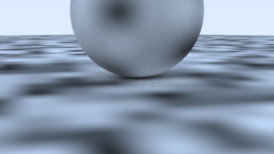
这会输出更平滑的图像:
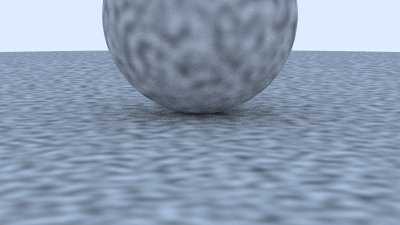
5.4. 调整频率 频率也有点低。我们可以缩放输入点,使其变化得更快。
1 2 3 4 5 6 7 8 9 10 11 12 class noise_texture : public texture { public : noise_texture (double scale) : scale (scale) {} color value (double u, double v, const point3& p) const override { return color (1 ,1 ,1 ) * noise.noise (scale * p); } private : perlin noise; double scale; };
然后我们将该比例添加到perlin_spheres()场景描述中:
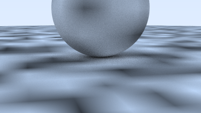
1 2 3 4 5 6 7 8 9 void perlin_spheres () ... auto pertext = make_shared <noise_texture>(4 ); world.add (make_shared <sphere>(point3 (0 ,-1000 ,0 ), 1000 , make_shared <lambertian>(pertext))); world.add (make_shared <sphere>(point3 (0 , 2 , 0 ), 2 , make_shared <lambertian>(pertext))); camera cam; ... }
渲染效果如下:
5.5. 在格点上使用随机向量 这看起来仍然有点块状,可能是因为图案的最小值和最大值总是恰好落在整数x/y/z上。Ken Perlin 非常聪明的技巧是将随机单位向量(而不仅仅是浮点数)放在格点上,并使用点积将最小值和最大值移出格点。因此,我们需要将随机浮点数更改为随机向量。这些向量是合理的不规则方向集,我不会费心使它们完全均匀:
1 2 3 4 5 6 7 8 9 10 11 12 13 14 15 16 17 18 19 20 21 22 class perlin { public : perlin () { for (int i = 0 ; i < point_count; i++) { randvec[i] = unit_vector (vec3::random (-1 ,1 )); } perlin_generate_perm (perm_x); perlin_generate_perm (perm_y); perlin_generate_perm (perm_z); } ... private : static const int point_count = 256 ; vec3 randvec[point_count]; int perm_x[point_count]; int perm_y[point_count]; int perm_z[point_count]; ... };
Perlin类的noise()方法现在改成:
1 2 3 4 5 6 7 8 9 10 11 12 13 14 15 16 17 18 19 20 21 22 23 24 25 26 27 class perlin { public : ... double noise (const point3& p) const auto u = p.x () - std::floor (p.x ()); auto v = p.y () - std::floor (p.y ()); auto w = p.z () - std::floor (p.z ()); auto i = int (std::floor (p.x ())); auto j = int (std::floor (p.y ())); auto k = int (std::floor (p.z ())); vec3 c[2 ][2 ][2 ]; for (int di=0 ; di < 2 ; di++) for (int dj=0 ; dj < 2 ; dj++) for (int dk=0 ; dk < 2 ; dk++) c[di][dj][dk] = randvec[perm_x[(i+di) & 255 ] ^ perm_y[(j+dj) & 255 ] ^ perm_z[(k+dk) & 255 ] ]; return perlin_interp (c, u, v, w); } ... };
插值会变得稍微复杂一些:
1 2 3 4 5 6 7 8 9 10 11 12 13 14 15 16 17 18 19 20 21 22 23 24 25 26 27 class perlin { ... private : ... static double perlin_interp (const vec3 c[2 ][2 ][2 ], double u, double v, double w) auto uu = u*u*(3 -2 *u); auto vv = v*v*(3 -2 *v); auto ww = w*w*(3 -2 *w); auto accum = 0.0 ; for (int i=0 ; i < 2 ; i++) for (int j=0 ; j < 2 ; j++) for (int k=0 ; k < 2 ; k++) { vec3 weight_v (u-i, v-j, w-k) ; accum += (i*uu + (1 -i)*(1 -uu)) * (j*vv + (1 -j)*(1 -vv)) * (k*ww + (1 -k)*(1 -ww)) * dot (c[i][j][k], weight_v); } return accum; } };
Perlin插值函数可以返回负数。这些负数将会传给linear_to_gamma()函数,然而该函数只接受正值输入。为了解决这个问题,我们将会把它的值范围($(-1,1)$)映射到范围$(0,1)$。
1 2 3 4 5 6 7 8 9 10 11 12 class noise_texture : public texture { public : noise_texture (double scale) : scale (scale) {} color value (double u, double v, const point3& p) const override { return color (1 ,1 ,1 ) * 0.5 * (1.0 + noise.noise (scale * p)); } private : perlin noise; double scale; };
最终给出了一些更合理的结果:
5.6. 湍流 通常会使用具有多个复合频率的复合噪声。这通常称为湍流,是多次调用噪声的总和:=
1 2 3 4 5 6 7 8 9 10 11 12 13 14 15 16 17 18 19 20 21 22 23 24 class perlin { ... public : ... double noise (const point3& p) const ... } double turb (const point3& p, int depth) const auto accum = 0.0 ; auto temp_p = p; auto weight = 1.0 ; for (int i = 0 ; i < depth; i++) { accum += weight * noise (temp_p); weight *= 0.5 ; temp_p *= 2 ; } return std::fabs (accum); } ...
1 2 3 4 5 6 7 8 9 10 11 12 class noise_texture : public texture { public : noise_texture (double scale) : scale (scale) {} color value (double u, double v, const point3& p) const override { return color (1 ,1 ,1 ) * noise.turb (p, 7 ); } private : perlin noise; double scale; };
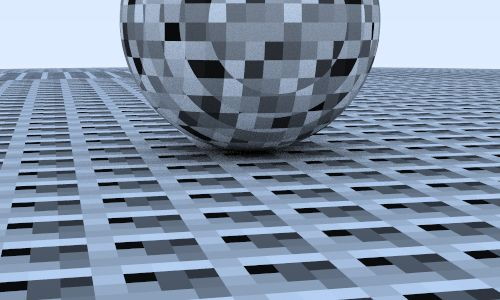
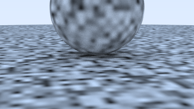
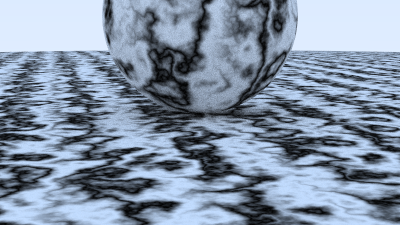
直接使用湍流,会产生一种保护网的外观:
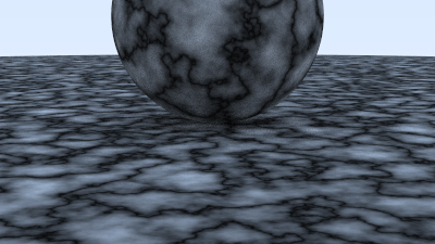
5.7. 调整相位 然而,湍流通常是间接使用的。例如,程序化实体纹理的“Hello World”是一个简单的大理石纹理。基本思想是使颜色与正弦函数成比例,并使用湍流来调整相位(因此它会在$sin(x)$中移动$x$),从而使条纹起伏不定。注释掉直线噪声和湍流,产生大理石般的效果的代码如下:
1 2 3 4 5 6 7 8 9 10 11 12 class noise_texture : public texture { public : noise_texture (double scale) : scale (scale) {} color value (double u, double v, const point3& p) const override { return color (.5 , .5 , .5 ) * (1 + std::sin (scale * p.z () + 10 * noise.turb (p, 7 ))); } private : perlin noise; double scale; };
渲染效果如下:
6. 四边形 我们已经完成了这三本系列书的一半以上,其中球体是我们唯一的几何图元,是时候添加我们的第二个图元了。
6.1. 四边形的定义 虽然我们将新图元命名为“四边形”,但从技术上讲,它将是平行四边形(对边平行),而不是一般的四边形。为了达到我们的目的,我们将使用三个几何实体来定义四边形:
$Q$,角点。
$u$,表示第一条边的向量。$Q+u$表示$Q$的一个临边。
$v$,表示第二条边的向量。$Q+v$ gives the other corner adjacent to $Q$.
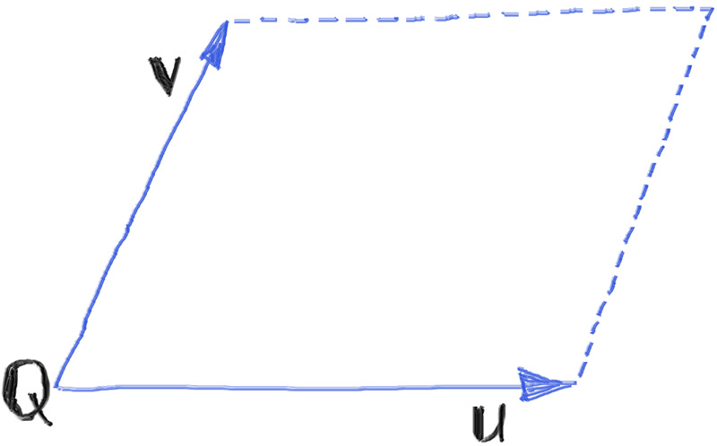
平行四边形中点Q的对角由$Q+u+v$给出。这些值是三维的,尽管四边形本身是二维对象。例如,一个四边形的角位于原点,在$Z$方向延伸两个单位,在$Y$方向延伸一个单位,则其值$Q=(0,0,0)$、$u=(0,0,2)$和$v=(0,1,0)$。
如下图所示,是平行四边形中$Q,u,v$的几何示意图。
四边形是扁平的,因此如果四边形位于$XY$、$YZ$或$ZX$平面,则其AABB在一个维度上的厚度为零。这可能会导致射线相交时出现数值问题,但我们可以将包围盒扩大一个微小的值,来解决这个问题。扩充是可以的,因为我们不会改变四边形的交点。我们只是扩大它,防止出现数值问题的可能性,而且包围盒只是对实际形状的粗略近似。为了解决这种情况,我们进行微小的扩充,以确保新构建的AABB始终具有非零体积:
1 2 3 4 5 6 7 8 9 10 11 12 13 14 15 16 17 18 19 20 21 22 23 24 25 26 27 28 29 30 31 32 33 34 35 ... class aabb { public : ... aabb (const interval& x, const interval& y, const interval& z) : x (x), y (y), z (z) { pad_to_minimums (); } aabb (const point3& a, const point3& b) { x = interval (std::fmin (a[0 ],b[0 ]), std::fmax (a[0 ],b[0 ])); y = interval (std::fmin (a[1 ],b[1 ]), std::fmax (a[1 ],b[1 ])); z = interval (std::fmin (a[2 ],b[2 ]), std::fmax (a[2 ],b[2 ])); pad_to_minimums (); } ... static const aabb empty, universe; private : void pad_to_minimums () double delta = 0.0001 ; if (x.size () < delta) x = x.expand (delta); if (y.size () < delta) y = y.expand (delta); if (z.size () < delta) z = z.expand (delta); } };
现在,我们就可以开始实现quad类了:
1 2 3 4 5 6 7 8 9 10 11 12 13 14 15 16 17 18 19 20 21 22 23 24 25 26 27 28 29 30 31 32 33 34 #ifndef QUAD_H #define QUAD_H #include "hittable.h" class quad : public hittable { public : quad (const point3& Q, const vec3& u, const vec3& v, shared_ptr<material> mat) : Q (Q), u (u), v (v), mat (mat) { set_bounding_box (); } virtual void set_bounding_box () auto bbox_diagonal1 = aabb (Q, Q + u + v); auto bbox_diagonal2 = aabb (Q + u, Q + v); bbox = aabb (bbox_diagonal1, bbox_diagonal2); } aabb bounding_box () const override { return bbox; } bool hit (const ray& r, interval ray_t , hit_record& rec) const override return false ; } private : point3 Q; vec3 u, v; shared_ptr<material> mat; aabb bbox; }; #endif
6.2. 射线与平面相交 正如前面看到的,quad::hit()还没有实现。就像球体一样,我们需要判断给定的射线与该四边形是否相交,如果相交,则填充hit_record中定义的那些变量(相交点,法线,纹理坐标等等)。
射线与四边形的相交分为以下三步:
找到包含该四边形的平面
求解射线与平面的相交点
判断相交点是否在四边形内。
我们首先解决中间步骤,解决射线与平面的相交问题。
球面通常是第一个教授的光线追踪的图元,因为它们的隐式公式使得求解射线相交变得非常容易。与球面一样,平面也有一个隐式公式,我们可以使用它们的隐式公式来生成求解射线与平面相交的算法。事实上,求解射线平面相交甚至比求解射线与球面相交更容易。
你可能已经知道这个平面的隐式公式:
其中$A,B,C,D$只是常数,而$x,y,z$是平面上任意点$(x,y,z)$的值。因此,平面是满足上述公式的所有点$(x,y,z)$的集合。使用替代公式会让事情稍微简单一些:
(我们没有翻转$D$的符号,因为它只是一些常数,换到右边只是变成了另一个常数,我们后续会对此进行解释。)
有一种直观的方式来理解这个公式:给定垂直于法线向量的平面$n=(A,B,C)$,以及位置向量$v=(x,y,z)$(即从原点到平面上任意一点的向量),那么我们可以使用点积来求解$D$:
对于平面上任意点。这是上面给出的$Ax+By+Cz=D$公式的等效公式,只是现在以向量的形式表示。代入射线公式$R(t) = P + td$,可得:
求解$t$:
有了$t$,带入射线方程可以算出相交点。注意,当射线与平面平行时,分母$n\cdot d$可能为零。在这种情况下,我们可以立即判断射线和平面是不相交的。
我们可以找到射线与包含给定四边形的平面之间的交点。事实上,我们可以把此方法推广到任何 平面图元上,如三角形和圆盘(稍后会详细介绍)。
6.3. 计算包含给定四边形的平面 我们已经解决了上面的第二步:假设我们有平面方程,则求解射线与平面的交点。为此,我们需要解决上面的第一步:找到包含四边形的平面的方程。我们有四边形参数$Q$、$u$和$v$,并且想要由这三个值推出的平面方程的参数。
幸运的是,这非常简单。回想一下,在方程$Ax+By+Cz=D$中,$(A,B,C)$表示法向量。为了得到法向量,我们只需计算两个边向量$u$和$v$的叉积即可:
满足方程$Ax+By+Cz=D$的所有点$(x,y,z)$构成一个平面。我们知道$Q$位于平面上,带入公式即可求解$D$:
将这些值添加到quad类:
1 2 3 4 5 6 7 8 9 10 11 12 13 14 15 16 17 18 19 20 21 class quad : public hittable { public : quad (const point3& Q, const vec3& u, const vec3& v, shared_ptr<material> mat) : Q (Q), u (u), v (v), mat (mat) { auto n = cross (u, v); normal = unit_vector (n); D = dot (normal, Q); set_bounding_box (); } ... private : point3 Q; vec3 u, v; shared_ptr<material> mat; aabb bbox; vec3 normal; double D; };
我们将会使用normal和D去计算包含四边形的平面和射线的交点。
让我们先实现hit()方法来处理射线与平面相交的问题,后续再逐步实现与四边形相交的逻辑。
1 2 3 4 5 6 7 8 9 10 11 12 13 14 15 16 17 18 19 20 21 22 23 24 25 26 27 class quad : public hittable { ... bool hit (const ray& r, interval ray_t , hit_record& rec) const override auto denom = dot (normal, r.direction ()); if (std::fabs (denom) < 1e-8 ) return false ; auto t = (D - dot (normal, r.origin ())) / denom; if (!ray_t .contains (t)) return false ; auto intersection = r.at (t); rec.t = t; rec.p = intersection; rec.mat = mat; rec.set_face_normal (r, normal); return true ; } ... }
6.4. 点在平面上的定位 在此阶段,交点位于包含四边形的平面上,但它可能位于平面上的任何位置:射线与平面交点将位于四边形的内部或外部。当交点位于四边形内部时,才能被接受,否则不可接受。为了确定点相对于四边形的位置,并计算交点的纹理坐标,我们需要在平面上定位交点。
为此,我们将为平面构建一个 坐标系 ——定位平面上任意点的方法。我们已经在3D空间中使用了坐标系——它由原点$O$和三个基向量$x$、$y$和$z$定义。
由于平面是二维结构,我们只需要一个平面原点$Q$ 和两个基向量:$u$和$v$。通常,轴是相互垂直的。但是并不总是需要,实际你只需要两个不平行的轴即可表示出平面上的所有点。
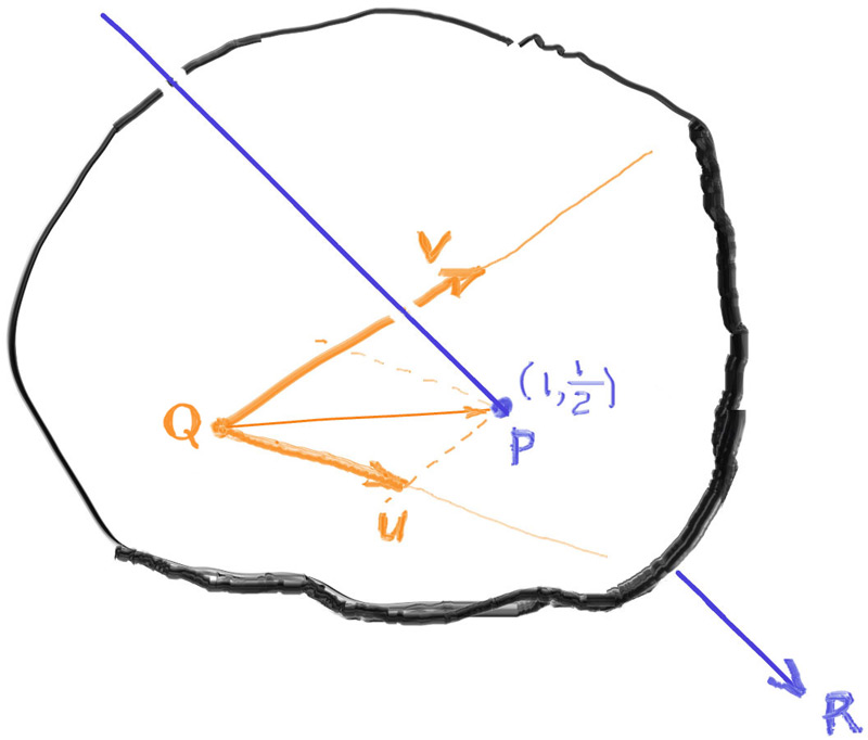
以上图为例(图6)。射线$R$与平面相交,可计算出交点$P$(不要与上面射线的起点混淆了)。以平面向量$u$和$v$为基准,上例中的交点$P$位于$Q+(1)u+(\frac{1}{2})v$。换句话说,交点$P$的$UV$(平面)坐标为$(1,\frac{1}{2})$。
一般地,给定某个任意点$P$,我们寻找两个标量值$\alpha$和$\beta$,可以用下面的公式来表示平面上的点:
这里首先给出平面坐标$\alpha$和$\beta$的方程,下一节再给出推导过程:
$p$和$w$的定义如下:
对于给定的四边形,向量$w$是常向量,因此我们可以提前计算该值:
1 2 3 4 5 6 7 8 9 10 11 12 13 14 15 16 17 18 19 20 21 22 23 24 class quad : public hittable { public : quad (const point3& Q, const vec3& u, const vec3& v, shared_ptr<material> mat) : Q (Q), u (u), v (v), mat (mat) { auto n = cross (u, v); normal = unit_vector (n); D = dot (normal, Q); w = n / dot (n,n); set_bounding_box (); } ... private : point3 Q; vec3 u, v; vec3 w; shared_ptr<material> mat; aabb bbox; vec3 normal; double D; };
6.5. 平面坐标公式 (本节介绍上述方程的推导。如果你不感兴趣,可以直接跳至下一部分。)
再回到图6。如果保证平面基向量$u$和$v$彼此正交(它们之间形成 90° 角),则求解$α$和$β$就是使用点积将$P$投影到每个基向量$u$ 和$v $的简单问题。但是,由于我们没有限制$u$和$v$正交,因此数学运算会稍微复杂一些。
首先,先看下面的公式:
上式中,$P$是交点,$p$是点$Q$到点$P$的向量。
分别计算$p$与$u$和$v$的叉积:
由于任何向量与自身的叉积为0,上述方程可以化简如下:
现在来求解系数$α$和$β$。如果你对向量数学不熟悉,你可能会尝试除以$u×v$和$v×u$,但你不能除以向量。不过,我们可以将上述等式的两边与平面法线 $n=u×v$进行点积,将两边简化为标量,然后我们就可以除以标量。
分离系数只是一个简单的除法问题,上式变形如下:
对$α$的分子和分母的叉积取反(数学中,$a×b=−b×a$)可以得到两个系数的共同分母:
现在我们可以进行最后的简化,计算一个向量$w$,对于平面内任意点$P$,该向量$w$对于该平面而言都是恒定的:
6.6. 使用平面坐标判断交点的内外 至此,我们已经可以计算出交点的平面坐标$\alpha$和$\beta$,我们可以使用这些来判断交点是位于四边形内部还是外部(前提是,射线与平面的交点存在)。
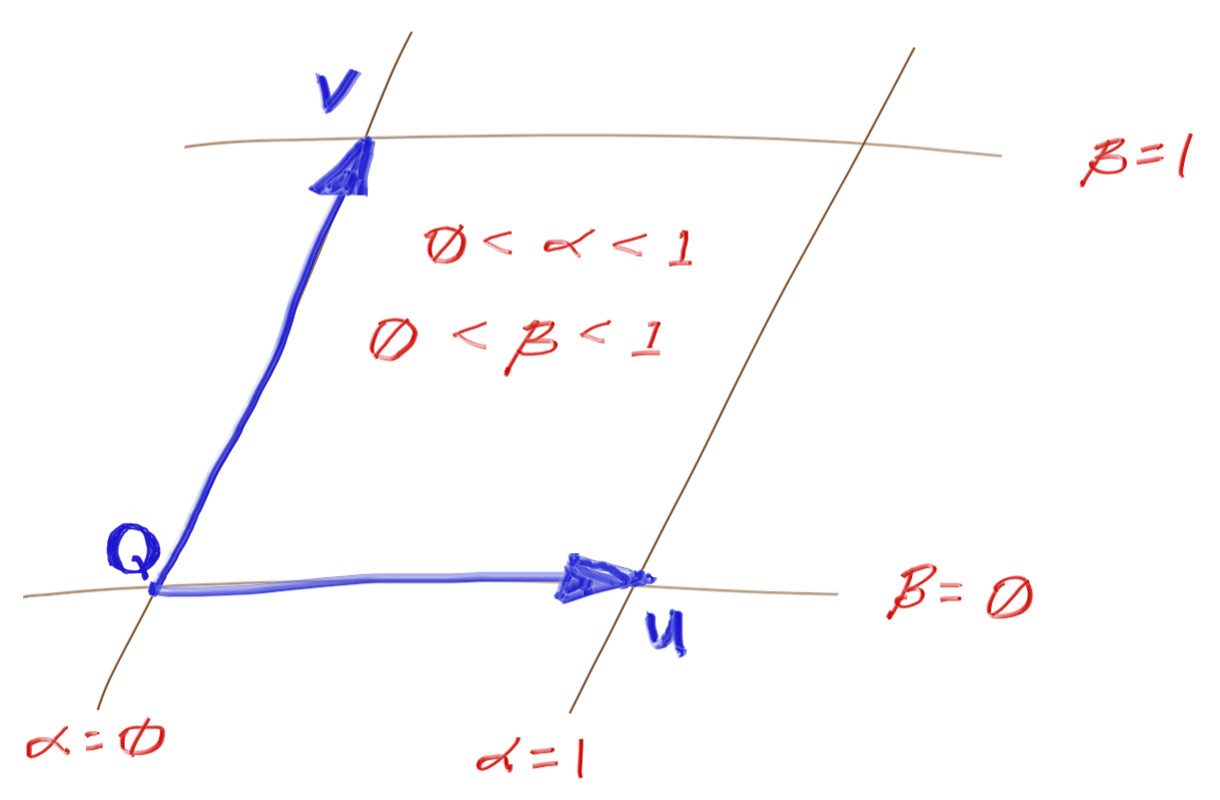
平面的坐标区域划分如下图所示:
因此,要判断平面坐标为$(α,β)$的点是否位于四边形内部,只需同时满足以下条件:
$0\leq\alpha\leq1$
$0\leq\beta\leq1$
这是实现四边形图元所需的最后一部分。
为了使这种实验更容易一些,我们将从hit()方法中分离出判断$(α,β)$方位的方法。
1 2 3 4 5 6 7 8 9 10 11 12 13 14 15 16 17 18 19 20 21 22 23 24 25 26 27 28 29 30 31 32 33 34 35 36 37 38 39 40 41 42 43 44 45 46 47 48 49 50 51 52 53 54 55 56 class quad : public hittable { public : ... bool hit (const ray& r, interval ray_t , hit_record& rec) const override auto denom = dot (normal, r.direction ()); if (std::fabs (denom) < 1e-8 ) return false ; auto t = (D - dot (normal, r.origin ())) / denom; if (!ray_t .contains (t)) return false ; auto intersection = r.at (t); vec3 planar_hitpt_vector = intersection - Q; auto alpha = dot (w, cross (planar_hitpt_vector, v)); auto beta = dot (w, cross (u, planar_hitpt_vector)); if (!is_interior (alpha, beta, rec)) return false ; rec.t = t; rec.p = intersection; rec.mat = mat; rec.set_face_normal (r, normal); return true ; } virtual bool is_interior (double a, double b, hit_record& rec) const interval unit_interval = interval (0 , 1 ); if (!unit_interval.contains (a) || !unit_interval.contains (b)) return false ; rec.u = a; rec.v = b; return true ; } private : point3 Q; vec3 u, v; vec3 w; shared_ptr<material> mat; aabb bbox; vec3 normal; double D; };
现在,让我们增加一个场景来测试我们新创建的四边形图元:
1 2 3 4 5 6 7 8 9 10 11 12 13 14 15 16 17 18 19 20 21 22 23 24 25 26 27 28 29 30 31 32 33 34 35 36 37 38 39 40 41 42 43 44 45 46 47 48 49 50 51 52 53 54 55 56 #include "rtweekend.h" #include "bvh.h" #include "camera.h" #include "hittable.h" #include "hittable_list.h" #include "material.h" #include "quad.h" #include "sphere.h" #include "texture.h" ... void quads () hittable_list world; auto left_red = make_shared <lambertian>(color (1.0 , 0.2 , 0.2 )); auto back_green = make_shared <lambertian>(color (0.2 , 1.0 , 0.2 )); auto right_blue = make_shared <lambertian>(color (0.2 , 0.2 , 1.0 )); auto upper_orange = make_shared <lambertian>(color (1.0 , 0.5 , 0.0 )); auto lower_teal = make_shared <lambertian>(color (0.2 , 0.8 , 0.8 )); world.add (make_shared <quad>(point3 (-3 ,-2 , 5 ), vec3 (0 , 0 ,-4 ), vec3 (0 , 4 , 0 ), left_red)); world.add (make_shared <quad>(point3 (-2 ,-2 , 0 ), vec3 (4 , 0 , 0 ), vec3 (0 , 4 , 0 ), back_green)); world.add (make_shared <quad>(point3 ( 3 ,-2 , 1 ), vec3 (0 , 0 , 4 ), vec3 (0 , 4 , 0 ), right_blue)); world.add (make_shared <quad>(point3 (-2 , 3 , 1 ), vec3 (4 , 0 , 0 ), vec3 (0 , 0 , 4 ), upper_orange)); world.add (make_shared <quad>(point3 (-2 ,-3 , 5 ), vec3 (4 , 0 , 0 ), vec3 (0 , 0 ,-4 ), lower_teal)); camera cam; cam.aspect_ratio = 1.0 ; cam.image_width = 400 ; cam.samples_per_pixel = 100 ; cam.max_depth = 50 ; cam.vfov = 80 ; cam.lookfrom = point3 (0 ,0 ,9 ); cam.lookat = point3 (0 ,0 ,0 ); cam.vup = vec3 (0 ,1 ,0 ); cam.defocus_angle = 0 ; cam.render (world); } int main () switch (5 ) { case 1 : bouncing_spheres (); break ; case 2 : checkered_spheres (); break ; case 3 : earth (); break ; case 4 : perlin_spheres (); break ; case 5 : quads (); break ; } }
6.7. 其他2D图元 看到这里,考虑一下你能够使用$(\alpha,\beta)$坐标来判断一个点是否在四边形(平行四边形)内,不难想象,使用相同的坐标也可以用来判断交点在其他2D图元中。
例如,假设我们改变is_interior()函数,在sqrt(a*a+b*b)<r的时候返回true。这就表示交点是否在一个圆内。
对于三角形,判断条件将会是:a>0 && b>0 && a+b < 1。
我们把其他2D图元的实现作为布置给读者的作业,你可以自由尝试去实现这些方案。您甚至可以根据纹理贴图或模型无限细分形状(Mandelbrot shape)的像素创建裁切模板!作为一个小彩蛋,请查看代码仓库中的“alternate-2D-primitives”标签。它包含“src/TheNextWeek/quad.h”中三角形、椭圆形和环形(环)的实现方案。
7. 光源 光照是光线追踪算法中很关键的部分。早期简单的光线跟踪渲染器使用抽象的光源,类似点光源,或者方向光。现代方法提出了基于物理的光源,它们有位置,有形状。为了创建这样的光源,我们需要使用一些规则的形状,作为会发光的灯加入我们的场景中。
7.1. 自发光材质 首先,让我们创造一个发光的材质。我们需要增加一个emitted函数()。类似背景,它仅仅需要告诉调用者它的颜色,并且不需要反射。这非常简单:
1 2 3 4 5 6 7 8 9 10 11 12 13 14 15 16 class dielectric : public material { ... } class diffuse_light : public material { public : diffuse_light (shared_ptr<texture> tex) : tex (tex) {} diffuse_light (const color& emit) : tex (make_shared <solid_color>(emit)) {} color emitted (double u, double v, const point3& p) const override { return tex->value (u, v, p); } private : shared_ptr<texture> tex; };
因此,我们没必要让那些非自发光材质射线emitted()方法,让基类返回黑色就好:
1 2 3 4 5 6 7 8 9 10 11 12 13 14 class material { public : virtual ~material () = default ; virtual color emitted (double u, double v, const point3& p) const return color (0 ,0 ,0 ); } virtual bool scatter ( const ray& r_in, const hit_record& rec, color& attenuation, ray& scattered ) const return false ; } };
7.2. 增加背景色 下一步,我们想要一个纯黑色背景,让场景中的光线来自于自发光物体。为了达到这个目的,我们将会为ray_color函数增加一个背景颜色的参数,并关注一个新的值:color_from_emission。
1 2 3 4 5 6 7 8 9 10 11 12 13 14 15 16 17 18 19 20 21 22 23 24 25 26 27 28 29 30 31 32 33 34 35 class camera { public : double aspect_ratio = 1.0 ; int image_width = 100 ; int samples_per_pixel = 10 ; int max_depth = 10 ; color background; ... private : ... color ray_color (const ray& r, int depth, const hittable& world) const { if (depth <= 0 ) return color (0 ,0 ,0 ); hit_record rec; if (!world.hit (r, interval (0.001 , infinity), rec)) return background; ray scattered; color attenuation; color color_from_emission = rec.mat->emitted (rec.u, rec.v, rec.p); if (!rec.mat->scatter (r, rec, attenuation, scattered)) return color_from_emission; color color_from_scatter = attenuation * ray_color (scattered, depth-1 , world); return color_from_emission + color_from_scatter; } };
在main()函数中,之前定义的场景里,定义background:
1 2 3 4 5 6 7 8 9 10 11 12 13 14 15 16 17 18 19 20 21 22 23 24 25 26 27 28 29 30 31 32 33 34 35 36 37 38 39 40 41 42 43 44 45 46 47 48 49 50 51 52 53 54 55 56 57 58 59 void bouncing_spheres () ... camera cam; cam.aspect_ratio = 16.0 / 9.0 ; cam.image_width = 400 ; cam.samples_per_pixel = 100 ; cam.max_depth = 20 ; cam.background = color (0.70 , 0.80 , 1.00 ); ... } void checkered_spheres () ... camera cam; cam.aspect_ratio = 16.0 / 9.0 ; cam.image_width = 400 ; cam.samples_per_pixel = 100 ; cam.max_depth = 50 ; cam.background = color (0.70 , 0.80 , 1.00 ); ... } void earth () ... camera cam; cam.aspect_ratio = 16.0 / 9.0 ; cam.image_width = 400 ; cam.samples_per_pixel = 100 ; cam.max_depth = 50 ; cam.background = color (0.70 , 0.80 , 1.00 ); ... } void perlin_spheres () ... camera cam; cam.aspect_ratio = 16.0 / 9.0 ; cam.image_width = 400 ; cam.samples_per_pixel = 100 ; cam.max_depth = 50 ; cam.background = color (0.70 , 0.80 , 1.00 ); ... } void quads () ... camera cam; cam.aspect_ratio = 1.0 ; cam.image_width = 400 ; cam.samples_per_pixel = 100 ; cam.max_depth = 50 ; cam.background = color (0.70 , 0.80 , 1.00 ); ... }
由于我们去掉了之前定义天空颜色的代码,因此我们在旧场景中,我们需要一个新的颜色来代替它。我们将整个天空保持为纯蓝白色。您可以随时传入布尔值以在之前的天空盒代码和新的纯色背景之间切换。我们在这里还是保持简洁。
7.3. 把物体变成光源 如果我们把一个矩形物体变成光源:
1 2 3 4 5 6 7 8 9 10 11 12 13 14 15 16 17 18 19 20 21 22 23 24 25 26 27 28 29 30 31 32 33 34 35 36 37 38 void simple_light () hittable_list world; auto pertext = make_shared <noise_texture>(4 ); world.add (make_shared <sphere>(point3 (0 ,-1000 ,0 ), 1000 , make_shared <lambertian>(pertext))); world.add (make_shared <sphere>(point3 (0 ,2 ,0 ), 2 , make_shared <lambertian>(pertext))); auto difflight = make_shared <diffuse_light>(color (4 ,4 ,4 )); world.add (make_shared <quad>(point3 (3 ,1 ,-2 ), vec3 (2 ,0 ,0 ), vec3 (0 ,2 ,0 ), difflight)); camera cam; cam.aspect_ratio = 16.0 / 9.0 ; cam.image_width = 400 ; cam.samples_per_pixel = 100 ; cam.max_depth = 50 ; cam.background = color (0 ,0 ,0 ); cam.vfov = 20 ; cam.lookfrom = point3 (26 ,3 ,6 ); cam.lookat = point3 (0 ,2 ,0 ); cam.vup = vec3 (0 ,1 ,0 ); cam.defocus_angle = 0 ; cam.render (world); } int main () switch (6 ) { case 1 : bouncing_spheres (); break ; case 2 : checkered_spheres (); break ; case 3 : earth (); break ; case 4 : perlin_spheres (); break ; case 5 : quads (); break ; case 6 : simple_light (); break ; } }
渲染结果如下:
注意到,灯光的强度大于$(1,1,1)$。这使得它足够明亮,可以照亮物体。
试着制作一些球形灯。
1 2 3 4 5 6 7 void simple_light () ... auto difflight = make_shared <diffuse_light>(color (4 ,4 ,4 )); world.add (make_shared <sphere>(point3 (0 ,7 ,0 ), 2 , difflight)); world.add (make_shared <quad>(point3 (3 ,1 ,-2 ), vec3 (2 ,0 ,0 ), vec3 (0 ,2 ,0 ), difflight)); ... }
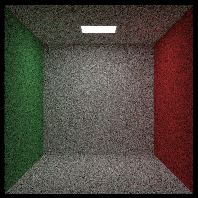
7.4. 创建一个空的”康奈尔盒子“ “康奈尔盒子”于1984年问世,用于模拟漫反射表面之间的光相互作用。让我们制作盒子的5面墙和灯光:
1 2 3 4 5 6 7 8 9 10 11 12 13 14 15 16 17 18 19 20 21 22 23 24 25 26 27 28 29 30 31 32 33 34 35 36 37 38 39 40 41 42 43 44 void cornell_box () hittable_list world; auto red = make_shared <lambertian>(color (.65 , .05 , .05 )); auto white = make_shared <lambertian>(color (.73 , .73 , .73 )); auto green = make_shared <lambertian>(color (.12 , .45 , .15 )); auto light = make_shared <diffuse_light>(color (15 , 15 , 15 )); world.add (make_shared <quad>(point3 (555 ,0 ,0 ), vec3 (0 ,555 ,0 ), vec3 (0 ,0 ,555 ), green)); world.add (make_shared <quad>(point3 (0 ,0 ,0 ), vec3 (0 ,555 ,0 ), vec3 (0 ,0 ,555 ), red)); world.add (make_shared <quad>(point3 (343 , 554 , 332 ), vec3 (-130 ,0 ,0 ), vec3 (0 ,0 ,-105 ), light)); world.add (make_shared <quad>(point3 (0 ,0 ,0 ), vec3 (555 ,0 ,0 ), vec3 (0 ,0 ,555 ), white)); world.add (make_shared <quad>(point3 (555 ,555 ,555 ), vec3 (-555 ,0 ,0 ), vec3 (0 ,0 ,-555 ), white)); world.add (make_shared <quad>(point3 (0 ,0 ,555 ), vec3 (555 ,0 ,0 ), vec3 (0 ,555 ,0 ), white)); camera cam; cam.aspect_ratio = 1.0 ; cam.image_width = 600 ; cam.samples_per_pixel = 200 ; cam.max_depth = 50 ; cam.background = color (0 ,0 ,0 ); cam.vfov = 40 ; cam.lookfrom = point3 (278 , 278 , -800 ); cam.lookat = point3 (278 , 278 , 0 ); cam.vup = vec3 (0 ,1 ,0 ); cam.defocus_angle = 0 ; cam.render (world); } int main () switch (7 ) { case 1 : bouncing_spheres (); break ; case 2 : checkered_spheres (); break ; case 3 : earth (); break ; case 4 : perlin_spheres (); break ; case 5 : quads (); break ; case 6 : simple_light (); break ; case 7 : cornell_box (); break ; } }
渲染结果如下:
由于灯光很小,所以这张图片的噪点非常多,大多数随机射线没有打到光源。
8. 实例 康奈尔盒子里经常还有两个方块。它们与墙有一个相对的旋转。首先,让我们创建一个返回的盒子的函数,它创建一个六个矩形组成的hittable_list:
1 2 3 4 5 6 7 8 9 10 11 12 13 14 15 16 17 18 19 20 21 22 23 24 25 26 27 28 29 30 #include "hittable.h" #include "hittable_list.h" class quad : public hittable { ... }; inline shared_ptr<hittable_list> box (const point3& a, const point3& b, shared_ptr<material> mat) auto sides = make_shared <hittable_list>(); auto min = point3 (std::fmin (a.x (),b.x ()), std::fmin (a.y (),b.y ()), std::fmin (a.z (),b.z ())); auto max = point3 (std::fmax (a.x (),b.x ()), std::fmax (a.y (),b.y ()), std::fmax (a.z (),b.z ())); auto dx = vec3 (max.x () - min.x (), 0 , 0 ); auto dy = vec3 (0 , max.y () - min.y (), 0 ); auto dz = vec3 (0 , 0 , max.z () - min.z ()); sides->add (make_shared <quad>(point3 (min.x (), min.y (), max.z ()), dx, dy, mat)); sides->add (make_shared <quad>(point3 (max.x (), min.y (), max.z ()), -dz, dy, mat)); sides->add (make_shared <quad>(point3 (max.x (), min.y (), min.z ()), -dx, dy, mat)); sides->add (make_shared <quad>(point3 (min.x (), min.y (), min.z ()), dz, dy, mat)); sides->add (make_shared <quad>(point3 (min.x (), max.y (), max.z ()), dx, -dz, mat)); sides->add (make_shared <quad>(point3 (min.x (), min.y (), min.z ()), dx, dz, mat)); return sides; }
然后,我们可以添加两个盒子到场景中(不带旋转)。
1 2 3 4 5 6 7 8 9 10 11 12 13 14 15 void cornell_box () ... world.add (make_shared <quad>(point3 (555 ,0 ,0 ), vec3 (0 ,555 ,0 ), vec3 (0 ,0 ,555 ), green)); world.add (make_shared <quad>(point3 (0 ,0 ,0 ), vec3 (0 ,555 ,0 ), vec3 (0 ,0 ,555 ), red)); world.add (make_shared <quad>(point3 (343 , 554 , 332 ), vec3 (-130 ,0 ,0 ), vec3 (0 ,0 ,-105 ), light)); world.add (make_shared <quad>(point3 (0 ,0 ,0 ), vec3 (555 ,0 ,0 ), vec3 (0 ,0 ,555 ), white)); world.add (make_shared <quad>(point3 (555 ,555 ,555 ), vec3 (-555 ,0 ,0 ), vec3 (0 ,0 ,-555 ), white)); world.add (make_shared <quad>(point3 (0 ,0 ,555 ), vec3 (555 ,0 ,0 ), vec3 (0 ,555 ,0 ), white)); world.add (box (point3 (130 , 0 , 65 ), point3 (295 , 165 , 230 ), white)); world.add (box (point3 (265 , 0 , 295 ), point3 (430 , 330 , 460 ), white)); camera cam; ... }
渲染结果如下:
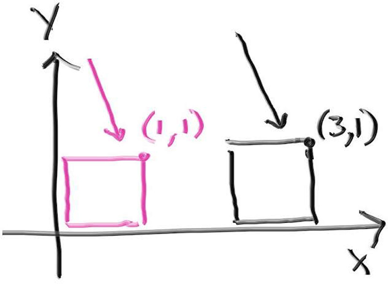
这样一来,我们就有盒子了,我们需要渲染它们,让它们更像康奈尔盒子。在光线追踪中,这通常通过实例完成。“实例”是指放置在场景中几何图元的副本。实例彼此之间相互独立,并且可以移动和旋转。在这个例子中,我们的几何图元就是可碰撞的box物体,并且我们想要旋转它。这在光线追踪中尤其容易,因为我们实际上不需要在场景中移动物体。相反,我们让光线像相反的方向移动。例如下图,可以设想一下物体有一个位移。我们可以让粉色盒子的每一个顶点的X值加2,让它从原来的位置往X轴正方形平移2个单位长度,也可以让盒子停留在原地,让射线的起点往X轴的负方向平移2个单位。(在光线跟踪中,我经常这么做)。
8.1. 实例的平移 你认为这是移动或坐标变化都可以。实现的方法是首先将射线向后移动偏移量,判断是否发生交点,然后再将该交点向前移动相同的偏移量。
我们需要将交点再次移动相同的偏移量,以便交点实际上位于原始射线的路径上。如果我们忘记平移交点,那么交点将偏离射线的路径,这是不正确的。让我们添加代码来实现这一点。
1 2 3 4 5 6 7 8 9 10 11 12 13 14 15 16 17 18 19 20 21 22 23 24 class hittable { ... }; class translate : public hittable { public : bool hit (const ray& r, interval ray_t , hit_record& rec) const override ray offset_r (r.origin() - offset, r.direction(), r.time()) ; if (!object->hit (offset_r, ray_t , rec)) return false ; rec.p += offset; return true ; } private : shared_ptr<hittable> object; vec3 offset; };
然后,实现translate类的其余部分:
1 2 3 4 5 6 7 8 9 10 11 12 13 14 class translate : public hittable { public : translate (shared_ptr<hittable> object, const vec3& offset) : object (object), offset (offset) { bbox = object->bounding_box () + offset; } bool hit (const ray& r, interval ray_t , hit_record& rec) const override ... } aabb bounding_box () const override { return bbox; } private : shared_ptr<hittable> object; vec3 offset; aabb bbox;};
此外,物体的包围盒也是需要平移的,否则可能会被包围盒误判为不相交。为了达到这个目的,可以实现表达式object->bounding_box() + offset。
1 2 3 4 5 6 7 8 9 10 11 12 13 14 class aabb { ... }; const aabb aabb::empty = aabb (interval::empty, interval::empty, interval::empty);const aabb aabb::universe = aabb (interval::universe, interval::universe, interval::universe);aabb operator +(const aabb& bbox, const vec3& offset) { return aabb (bbox.x + offset.x (), bbox.y + offset.y (), bbox.z + offset.z ()); } aabb operator +(const vec3& offset, const aabb& bbox) { return bbox + offset; }
由于aabb的每个维度都被表示为一个interval,我们也需要一个新的运算符来扩展interval。
1 2 3 4 5 6 7 8 9 10 11 12 13 14 class interval { ... }; const interval interval::empty = interval (+infinity, -infinity);const interval interval::universe = interval (-infinity, +infinity);interval operator +(const interval& ival, double displacement) { return interval (ival.min + displacement, ival.max + displacement); } interval operator +(double displacement, const interval& ival) { return ival + displacement; }
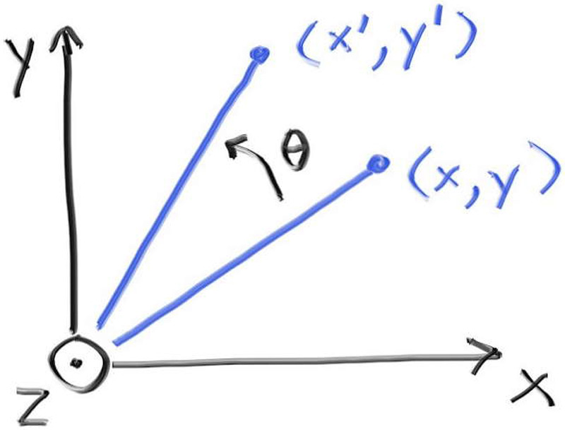
8.2. 实例旋转 旋转就不那么容易理解了,而且公式也比较复杂。图形学中常用的策略是应用所有关于$x$、$y$和$z$轴的旋转。这些旋转在某种意义上是轴对齐的。首先,让我们绕$z$轴旋转$\theta$。这将仅改变$x$和$y$,并且以不依赖于$z$的方式进行。
这涉及到一些基本的三角变换公式,这里就不多讲了(译者注:可以从单位圆的参数方程,推导这些公式 )。它有点绕,但很直观,你可以在任何图形学资料和许多讲义中找到它。绕$z$轴逆时针旋转的结果是:
它适用于任何$\theta$,并且不需要任何类似象限的东西。向相反的方向旋转,只需要把$\theta$取反即可,公式非常简单。
类似地,对于绕 y 旋转(就像我们想要对盒子中的块所做的那样),公式为:
绕X轴旋转的公式为:
将平移作为初始射线的简单位移是一个好主意。但是,对于像旋转这样更复杂的操作,很容易意外地弄错术语(或忘记负号),因此最好将旋转视为坐标的变化。
上面的translate::hit函数的伪代码从平移的角度描述了该函数:
将射线反向移动offset的距离
判断平移后的射线与物体是否相交(如果相交,计算交点)
将相交点正向平移offset的距离
这里也可以从”坐标变换”的角度来考虑这个过程:
将射线从世界空间转到对象空间
再对象空间判断是否相交(如果相交,计算对象空间的交点)
将交点转到世界空间
旋转物体不仅会改变交点,还会改变表面法线向量,从而改变反射和折射的方向。所以我们也需要改变法线。幸运的是,法线会像向量一样旋转,所以我们可以使用与上面相同的公式。虽然对于正在旋转和平移的物体,法线和向量可能看起来相同,但对于正在缩放的物体,需要特别注意保持法线与表面正交。我们不会在这里介绍这一点,但如果你要实现缩放,可以自己研究表面法线变换。
我们需要将射线从世界空间转到对象空间,对于旋转,意味着旋转$-\theta$
我们现在创建一个类来实现y-rotation。首先实现hit函数:
1 2 3 4 5 6 7 8 9 10 11 12 13 14 15 16 17 18 19 20 21 22 23 24 25 26 27 28 29 30 31 32 33 34 35 36 37 38 39 40 41 42 43 44 45 46 47 class translate : public hittable { ... }; class rotate_y : public hittable { public : bool hit (const ray& r, interval ray_t , hit_record& rec) const override auto origin = point3 ( (cos_theta * r.origin ().x ()) - (sin_theta * r.origin ().z ()), r.origin ().y (), (sin_theta * r.origin ().x ()) + (cos_theta * r.origin ().z ()) ); auto direction = vec3 ( (cos_theta * r.direction ().x ()) - (sin_theta * r.direction ().z ()), r.direction ().y (), (sin_theta * r.direction ().x ()) + (cos_theta * r.direction ().z ()) ); ray rotated_r (origin, direction, r.time()) ; if (!object->hit (rotated_r, ray_t , rec)) return false ; rec.p = point3 ( (cos_theta * rec.p.x ()) + (sin_theta * rec.p.z ()), rec.p.y (), (-sin_theta * rec.p.x ()) + (cos_theta * rec.p.z ()) ); rec.normal = vec3 ( (cos_theta * rec.normal.x ()) + (sin_theta * rec.normal.z ()), rec.normal.y (), (-sin_theta * rec.normal.x ()) + (cos_theta * rec.normal.z ()) ); return true ; } };
接着实现余下的部分:
1 2 3 4 5 6 7 8 9 10 11 12 13 14 15 16 17 18 19 20 21 22 23 24 25 26 27 28 29 30 31 32 33 34 35 36 37 38 39 40 41 42 43 44 45 46 class rotate_y : public hittable { public : rotate_y (shared_ptr<hittable> object, double angle) : object (object) { auto radians = degrees_to_radians (angle); sin_theta = std::sin (radians); cos_theta = std::cos (radians); bbox = object->bounding_box (); point3 min ( infinity, infinity, infinity) ; point3 max (-infinity, -infinity, -infinity) ; for (int i = 0 ; i < 2 ; i++) { for (int j = 0 ; j < 2 ; j++) { for (int k = 0 ; k < 2 ; k++) { auto x = i*bbox.x.max + (1 -i)*bbox.x.min; auto y = j*bbox.y.max + (1 -j)*bbox.y.min; auto z = k*bbox.z.max + (1 -k)*bbox.z.min; auto newx = cos_theta*x + sin_theta*z; auto newz = -sin_theta*x + cos_theta*z; vec3 tester (newx, y, newz) ; for (int c = 0 ; c < 3 ; c++) { min[c] = std::fmin (min[c], tester[c]); max[c] = std::fmax (max[c], tester[c]); } } } } bbox = aabb (min, max); } bool hit (const ray& r, interval ray_t , hit_record& rec) const override ... } aabb bounding_box () const override { return bbox; } private : shared_ptr<hittable> object; double sin_theta; double cos_theta; aabb bbox; };
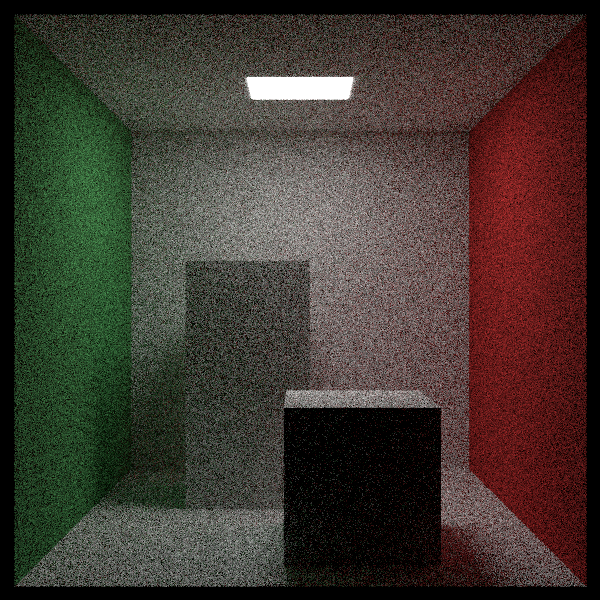
将这些修改应用到康奈尔盒子:
1 2 3 4 5 6 7 8 9 10 11 12 13 14 15 16 17 void cornell_box () ... world.add (make_shared <quad>(point3 (0 ,0 ,555 ), vec3 (555 ,0 ,0 ), vec3 (0 ,555 ,0 ), white)); shared_ptr<hittable> box1 = box (point3 (0 ,0 ,0 ), point3 (165 ,330 ,165 ), white); box1 = make_shared <rotate_y>(box1, 15 ); box1 = make_shared <translate>(box1, vec3 (265 ,0 ,295 )); world.add (box1); shared_ptr<hittable> box2 = box (point3 (0 ,0 ,0 ), point3 (165 ,165 ,165 ), white); box2 = make_shared <rotate_y>(box2, -18 ); box2 = make_shared <translate>(box2, vec3 (130 ,0 ,65 )); world.add (box2); camera cam; ... }
渲染结果如下:
9. 体积 烟雾/雾气/薄雾是光线追踪器中值得添加的功能之一。这些有时被称为体积 或参与介质 。另一个值得添加的功能是次表面散射,它有点像物体内部的浓雾。这通常会导致软件架构混乱,因为体积与表面不同,但有一种技巧是将体积变成随机表面。一堆烟雾可以用一个表面代替,该表面在体积的每个点上都可能存在,也可能不存在。这些内容,你看代码可能更好理解。
9.1. 恒密度介质 让我们从恒密度介质开始。射线穿过时有的会散射进入体积内,有的会直接穿过整个体积,像下图中中间那根射线那样。越薄的透明体积(如薄雾)更有可能产生像中间这样的射线。体积的厚度就决定了射线穿过的可能性。
由于射线穿过体积,它可能会散射到其他任意位置。体积密度越大,则更有可能发生这种情况。射线在任意小距离ΔL内散射的概率为:
其中,$C$与体积的光密度成正比。如果你学过微分方程,对于一个随机数,你就会得到发生散射的距离。如果该距离超出体积,则没有“命中”。对于恒定体积,我们只需要密度$C$和它的边界。我将使用另一个hittable对象作为边界。
代码实现如下:
1 2 3 4 5 6 7 8 9 10 11 12 13 14 15 16 17 18 19 20 21 22 23 24 25 26 27 28 29 30 31 32 33 34 35 36 37 38 39 40 41 42 43 44 45 46 47 48 49 50 51 52 53 54 55 56 57 58 59 60 61 62 63 #ifndef CONSTANT_MEDIUM_H #define CONSTANT_MEDIUM_H #include "hittable.h" #include "material.h" #include "texture.h" class constant_medium : public hittable { public : constant_medium (shared_ptr<hittable> boundary, double density, shared_ptr<texture> tex) : boundary (boundary), neg_inv_density (-1 /density), phase_function (make_shared <isotropic>(tex)) {} constant_medium (shared_ptr<hittable> boundary, double density, const color& albedo) : boundary (boundary), neg_inv_density (-1 /density), phase_function (make_shared <isotropic>(albedo)) {} bool hit (const ray& r, interval ray_t , hit_record& rec) const override hit_record rec1, rec2; if (!boundary->hit (r, interval::universe, rec1)) return false ; if (!boundary->hit (r, interval (rec1. t+0.0001 , infinity), rec2)) return false ; if (rec1. t < ray_t .min) rec1. t = ray_t .min; if (rec2. t > ray_t .max) rec2. t = ray_t .max; if (rec1. t >= rec2. t) return false ; if (rec1. t < 0 ) rec1. t = 0 ; auto ray_length = r.direction ().length (); auto distance_inside_boundary = (rec2. t - rec1. t) * ray_length; auto hit_distance = neg_inv_density * std::log (random_double ()); if (hit_distance > distance_inside_boundary) return false ; rec.t = rec1. t + hit_distance / ray_length; rec.p = r.at (rec.t); rec.normal = vec3 (1 ,0 ,0 ); rec.front_face = true ; rec.mat = phase_function; return true ; } aabb bounding_box () const override { return boundary->bounding_box (); } private : shared_ptr<hittable> boundary; double neg_inv_density; shared_ptr<material> phase_function; }; #endif
各向同性的散射函数会选择一个均匀的随机方向:
1 2 3 4 5 6 7 8 9 10 11 12 13 14 15 16 17 18 19 class diffuse_light : public material { ... }; class isotropic : public material { public : isotropic (const color& albedo) : tex (make_shared <solid_color>(albedo)) {} isotropic (shared_ptr<texture> tex) : tex (tex) {} bool scatter (const ray& r_in, const hit_record& rec, color& attenuation, ray& scattered) const override { scattered = ray (rec.p, random_unit_vector (), r_in.time ()); attenuation = tex->value (rec.u, rec.v, rec.p); return true ; } private : shared_ptr<texture> tex; };
我们之所以要如此小心边界周围的逻辑,是因为我们需要确保它适用于起点位于体积内的射线。在云层中,光线会大量反弹,所以这是一种常见情况。
此外,上面的代码存在一个假设:射线一旦离开了常密度边界,它就会永远在边界之外。换句话说,它假设边界形状是凸多边形。因此,这种特定的实现同样适用于像盒子或球体这样的边界形状,但不适用于圆环或包含空隙的形状。对于任意形状的边界的支持,我们将把它作为读者的课后作业。
(译者注:不支持任意形状的边界,是因为有镂空的物体,射线起点在镂空处时,rec1和rec2可能会射向自己,且方向相反,要避免这种情况。 )
9.2. 渲染带有烟和雾效果的康奈尔盒子 如果我们用烟和雾(暗粒子和亮粒子)替换这两个块,并使光变得更大(并且更暗,避免场景过曝),以实现更快的收敛:
1 2 3 4 5 6 7 8 9 10 11 12 13 14 15 16 17 18 19 20 21 22 23 24 25 26 27 28 29 30 31 32 33 34 35 36 37 38 39 40 41 42 43 44 45 46 47 48 49 50 51 52 53 54 55 56 57 58 59 60 61 62 63 64 65 66 67 68 #include "bvh.h" #include "camera.h" #include "constant_medium.h" #include "hittable.h" #include "hittable_list.h" #include "material.h" #include "quad.h" #include "sphere.h" #include "texture.h" ... void cornell_smoke () hittable_list world; auto red = make_shared <lambertian>(color (.65 , .05 , .05 )); auto white = make_shared <lambertian>(color (.73 , .73 , .73 )); auto green = make_shared <lambertian>(color (.12 , .45 , .15 )); auto light = make_shared <diffuse_light>(color (7 , 7 , 7 )); world.add (make_shared <quad>(point3 (555 ,0 ,0 ), vec3 (0 ,555 ,0 ), vec3 (0 ,0 ,555 ), green)); world.add (make_shared <quad>(point3 (0 ,0 ,0 ), vec3 (0 ,555 ,0 ), vec3 (0 ,0 ,555 ), red)); world.add (make_shared <quad>(point3 (113 ,554 ,127 ), vec3 (330 ,0 ,0 ), vec3 (0 ,0 ,305 ), light)); world.add (make_shared <quad>(point3 (0 ,555 ,0 ), vec3 (555 ,0 ,0 ), vec3 (0 ,0 ,555 ), white)); world.add (make_shared <quad>(point3 (0 ,0 ,0 ), vec3 (555 ,0 ,0 ), vec3 (0 ,0 ,555 ), white)); world.add (make_shared <quad>(point3 (0 ,0 ,555 ), vec3 (555 ,0 ,0 ), vec3 (0 ,555 ,0 ), white)); shared_ptr<hittable> box1 = box (point3 (0 ,0 ,0 ), point3 (165 ,330 ,165 ), white); box1 = make_shared <rotate_y>(box1, 15 ); box1 = make_shared <translate>(box1, vec3 (265 ,0 ,295 )); shared_ptr<hittable> box2 = box (point3 (0 ,0 ,0 ), point3 (165 ,165 ,165 ), white); box2 = make_shared <rotate_y>(box2, -18 ); box2 = make_shared <translate>(box2, vec3 (130 ,0 ,65 )); world.add (make_shared <constant_medium>(box1, 0.01 , color (0 ,0 ,0 ))); world.add (make_shared <constant_medium>(box2, 0.01 , color (1 ,1 ,1 ))); camera cam; cam.aspect_ratio = 1.0 ; cam.image_width = 600 ; cam.samples_per_pixel = 200 ; cam.max_depth = 50 ; cam.background = color (0 ,0 ,0 ); cam.vfov = 40 ; cam.lookfrom = point3 (278 , 278 , -800 ); cam.lookat = point3 (278 , 278 , 0 ); cam.vup = vec3 (0 ,1 ,0 ); cam.defocus_angle = 0 ; cam.render (world); } int main () switch (8 ) { case 1 : bouncing_spheres (); break ; case 2 : checkered_spheres (); break ; case 3 : earth (); break ; case 4 : perlin_spheres (); break ; case 5 : quads (); break ; case 6 : simple_light (); break ; case 7 : cornell_box (); break ; case 8 : cornell_smoke (); break ; } }
渲染结果如下:
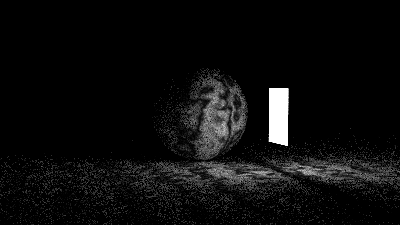
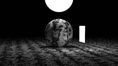
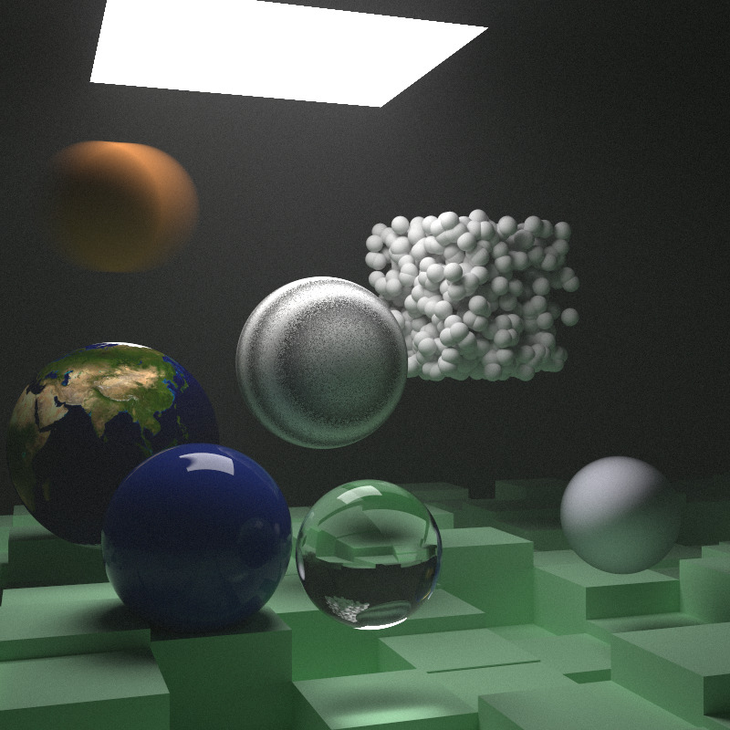
10. 最终场景 让我们把上面所有的内容放到一起,用一层薄薄的薄雾笼罩着一切。还有一个蓝色的次表面散射球(我们明确解释这一点,但电介质内部的体积就是次表面材料)。目前渲染器中最大的缺陷是没有阴影光线,但这就是我们自由获得焦散和次表面的原因,这是一个双刃剑的设计决定。
还要注意,我们将给这个最终场景增加参数,以支持较低质量的渲染,以便进行快速测试。
1 2 3 4 5 6 7 8 9 10 11 12 13 14 15 16 17 18 19 20 21 22 23 24 25 26 27 28 29 30 31 32 33 34 35 36 37 38 39 40 41 42 43 44 45 46 47 48 49 50 51 52 53 54 55 56 57 58 59 60 61 62 63 64 65 66 67 68 69 70 71 72 73 74 75 76 77 78 79 80 81 82 83 84 85 86 87 88 89 90 91 92 93 void final_scene (int image_width, int samples_per_pixel, int max_depth) hittable_list boxes1; auto ground = make_shared <lambertian>(color (0.48 , 0.83 , 0.53 )); int boxes_per_side = 20 ; for (int i = 0 ; i < boxes_per_side; i++) { for (int j = 0 ; j < boxes_per_side; j++) { auto w = 100.0 ; auto x0 = -1000.0 + i*w; auto z0 = -1000.0 + j*w; auto y0 = 0.0 ; auto x1 = x0 + w; auto y1 = random_double (1 ,101 ); auto z1 = z0 + w; boxes1. add (box (point3 (x0,y0,z0), point3 (x1,y1,z1), ground)); } } hittable_list world; world.add (make_shared <bvh_node>(boxes1)); auto light = make_shared <diffuse_light>(color (7 , 7 , 7 )); world.add (make_shared <quad>(point3 (123 ,554 ,147 ), vec3 (300 ,0 ,0 ), vec3 (0 ,0 ,265 ), light)); auto center1 = point3 (400 , 400 , 200 ); auto center2 = center1 + vec3 (30 ,0 ,0 ); auto sphere_material = make_shared <lambertian>(color (0.7 , 0.3 , 0.1 )); world.add (make_shared <sphere>(center1, center2, 50 , sphere_material)); world.add (make_shared <sphere>(point3 (260 , 150 , 45 ), 50 , make_shared <dielectric>(1.5 ))); world.add (make_shared <sphere>( point3 (0 , 150 , 145 ), 50 , make_shared <metal>(color (0.8 , 0.8 , 0.9 ), 1.0 ) )); auto boundary = make_shared <sphere>(point3 (360 ,150 ,145 ), 70 , make_shared <dielectric>(1.5 )); world.add (boundary); world.add (make_shared <constant_medium>(boundary, 0.2 , color (0.2 , 0.4 , 0.9 ))); boundary = make_shared <sphere>(point3 (0 ,0 ,0 ), 5000 , make_shared <dielectric>(1.5 )); world.add (make_shared <constant_medium>(boundary, .0001 , color (1 ,1 ,1 ))); auto emat = make_shared <lambertian>(make_shared <image_texture>("earthmap.jpg" )); world.add (make_shared <sphere>(point3 (400 ,200 ,400 ), 100 , emat)); auto pertext = make_shared <noise_texture>(0.2 ); world.add (make_shared <sphere>(point3 (220 ,280 ,300 ), 80 , make_shared <lambertian>(pertext))); hittable_list boxes2; auto white = make_shared <lambertian>(color (.73 , .73 , .73 )); int ns = 1000 ; for (int j = 0 ; j < ns; j++) { boxes2. add (make_shared <sphere>(point3::random (0 ,165 ), 10 , white)); } world.add (make_shared <translate>( make_shared <rotate_y>( make_shared <bvh_node>(boxes2), 15 ), vec3 (-100 ,270 ,395 ) ) ); camera cam; cam.aspect_ratio = 1.0 ; cam.image_width = image_width; cam.samples_per_pixel = samples_per_pixel; cam.max_depth = max_depth; cam.background = color (0 ,0 ,0 ); cam.vfov = 40 ; cam.lookfrom = point3 (478 , 278 , -600 ); cam.lookat = point3 (278 , 278 , 0 ); cam.vup = vec3 (0 ,1 ,0 ); cam.defocus_angle = 0 ; cam.render (world); } int main () switch (9 ) { case 1 : bouncing_spheres (); break ; case 2 : checkered_spheres (); break ; case 3 : earth (); break ; case 4 : perlin_spheres (); break ; case 5 : quads (); break ; case 6 : simple_light (); break ; case 7 : cornell_box (); break ; case 8 : cornell_smoke (); break ; case 9 : final_scene (800 , 10000 , 40 ); break ; default : final_scene (400 , 250 , 4 ); break ; } }
以每个像素10000根射线来渲染这个场景,将会产生如下的结果:(睡一觉再起来看)
现在就去制作一幅属于你自己的非常酷的图像吧!请参阅我们作品的 wiki 页面 ,获取更多与项目相关的资源。欢迎将问题、评论和精美图片通过电子邮件发送给我——ptrshrl@gmail.com
译者:寒江雪
转载请注明来源,欢迎对文章中的引用来源进行考证,欢迎指出任何有错误或不够清晰的表达。可以邮件